

MBTR
MBTR fits gradient-boosted trees with multivariate and structured responses, including shared-tree multilabel classification. Unlike fitting one independent model per output, a leaf may use a coupled response: a smoothed vector, a Fourier basis, a latent linear map, a set of quantiles, a ridge-linear model, or a vector of Bernoulli-logit updates.
The v0.2 implementation defines explicit contracts for split construction, optional post-structure refitting, and reported metrics, enforces tree-size invariants, and provides a compact scikit-learn-style estimator interface.
What's new in v0.2.0
This release substantially improves correctness, usability, and performance:
- Corrects split-gain, partition, minimum-leaf, validation, Fourier, and structured-objective defects while preserving the published hybrid quantile fitting strategy.
- Introduces the scikit-learn-style
MBTRegressorand the new binary/multilabelMBTClassifier, including constant, ridge-linear, and linear-logistic leaf responses with validation-based early stopping. - Adds verified NumPy and optional Numba engines, batched histogram split
search, sibling-histogram reuse, compact trees, and faster prediction.
Controlled multivariate benchmarks show standard-fit speedups of up to about
10×with essentially unchanged predictive quality. - Expands automated tests, serialization checks, reproducible performance and scientific benchmarks, examples, migration guidance, and API documentation.
MBT and legacy parameter names remain available for one transition cycle.
Previously saved v0.1 models should be retrained; see the
migration guide.
Installation
Install the core NumPy/SciPy implementation:
python -m pip install mbtr
Optional dependencies are grouped by purpose:
python -m pip install "mbtr[fast]"       # optional acceleration dependencies
python -m pip install "mbtr[plot]"       # plotting and NetworkX export
python -m pip install "mbtr[examples]"   # external dataset examples
For a development checkout, use python -m pip install -e ".[dev,test,docs,benchmark]".
Offline quickstart
This example is deterministic and does not download data:
import numpy as np

from mbtr import MBTRegressor

rng = np.random.default_rng(7)
X = rng.normal(size=(600, 6))
Y = np.column_stack(
    (
        2.0 * X[:, 0] - X[:, 1],
        X[:, 0] + 0.5 * X[:, 2],
        -X[:, 1] + X[:, 3],
    )
) + 0.1 * rng.normal(size=(600, 3))

X_train, X_test = X[:500], X[500:]
Y_train, Y_test = Y[:500], Y[500:]

model = MBTRegressor(
    objective="squared_error",
    n_estimators=50,
    learning_rate=0.08,
    max_bins=32,
    min_samples_leaf=15,
    max_depth=4,
    random_state=7,
)
model.fit(X_train, Y_train)
Y_pred = model.predict(X_test)

print(Y_pred.shape)       # (100, 3)
print(model.score(X_test, Y_test))
Use an explicit validation set for early stopping:
model = MBTRegressor(
    n_estimators=300,
    early_stopping_rounds=20,
    random_state=7,
)
model.fit(X[:400], Y[:400], eval_set=(X[400:500], Y[400:500]))

print(model.best_iteration_)
print(model.evals_result_["validation"])
For chronological data, always construct an explicit time-ordered validation
set. validation_fraction performs a seeded random split and is not suitable
for forecasting unless random validation is scientifically justified.
Binary and multilabel classification
MBTClassifier accepts either a one-dimensional binary target or a
two-dimensional 0/1 multilabel indicator matrix. Tree partitions are shared
across labels. Without a response design, each leaf returns one constant logit
update per label; probabilities and hard labels are produced only after the
ensemble logits are passed through the sigmoid and decision threshold:
from mbtr import MBTClassifier

labels = np.column_stack(
    (
        X[:, 0] + X[:, 1] > 0.0,
        X[:, 1] - X[:, 2] > 0.25,
        X[:, 0] * X[:, 3] > 0.0,
    )
).astype(int)

classifier = MBTClassifier(
    n_estimators=50,
    learning_rate=0.08,
    max_depth=4,
    decision_threshold=0.5,
    random_state=7,
)
classifier.fit(X[:500], labels[:500])
probability = classifier.predict_proba(X[500:])
prediction = classifier.predict(X[500:])

print(probability.shape)  # (100, 3), positive-label probabilities
print(classifier.score(X[500:], labels[500:]))  # exact/subset accuracy
For a one-dimensional binary target, predict_proba follows the usual
two-column (P(class=0), P(class=1)) convention. For a multilabel target it
returns one positive-label probability per output. decision_function exposes
the corresponding raw logits, and evals_result_ records mean binary
cross-entropy.
The Bernoulli objective evaluates its loss, gradient, and curvature without subtracting probabilities that have rounded to one. This applies the numerical principle in Barron, Gnanapragasam, and Tschannen's “A Fix for Softmax and Cross-Entropy” to the binary case. The current classifier does not use softmax and does not yet accept multiclass targets. A future grouped-softmax implementation will require block Hessians and the paper's target-excluded, zero-sum construction.
Supplying response_features selects linear-logistic leaves. Each leaf then
fits one ridge-logit update per label as a linear function of the supplied
design, with an intercept added internally. The original X still controls
tree routing, so the split matrix and the within-leaf design can be different:
linear_classifier = MBTClassifier(
    n_estimators=50,
    linear_response_curvature="upper_bound",
    l2_regularization=1e-3,
    random_state=7,
)
linear_classifier.fit(
    X[:500],
    labels[:500],
    response_features=X[:500, :3],
)
probability = linear_classifier.predict_proba(
    X[500:],
    response_features=X[500:, :3],
)
The default linear_response_curvature="upper_bound" uses the global
Bernoulli curvature bound 1/4, allowing all labels to share one design Gram
matrix. "exact" instead builds a probability-weighted Gram matrix for every
label and boosting round. It can fit the local Newton geometry more closely,
but its time and temporary-memory costs grow with both the number of labels and
the square of the response-design width. The default therefore has roughly the
same matrix order as linear-response regression. Set
regularize_intercept=True only when the intercept should receive the ridge
penalty too.
Structured objectives
| Objective | Required configuration | Prediction shape |
|---|---|---|
squared_error (mse) |
none | (samples, outputs) |
time_smoother |
lambda_smooth |
(samples, outputs) |
fourier |
n_harmonics |
(samples, outputs) |
latent_variable |
S, precision |
(samples, outputs) |
linear_regression |
response_features in fit and predict |
(samples, outputs) |
quantile |
ordered alphas; optional smoothing |
(samples, outputs, quantiles) |
quadratic_quantile |
ordered alphas; optional quadratic_scale, denominator_floor |
(samples, outputs, quantiles) |
pseudo_huber_quantile |
ordered alphas; optional delta |
(samples, outputs, quantiles) |
Objective-specific settings belong in objective_params:
smooth_model = MBTRegressor(
    objective="time_smoother",
    objective_params={"lambda_smooth": 2.0},
)
The two published quantile objectives deliberately separate tree construction
from the statistical target. quantile uses logistic-smoothed derivatives for
split search, while quadratic_quantile uses the partition-dependent
linear–quadratic relaxation from the paper. Both initialize and, by default,
refit terminal responses with empirical residual quantiles, report pinball
loss, and apply monotonic step acceptance to pinball loss. Set
refit_leaves=False to retain the second-order leaf responses. The separate
pseudo_huber_quantile objective optimizes its smooth asymmetric pseudo-Huber
surrogate end to end.
Linear regression responses also use separate features for tree partitioning and the model inside each leaf:
linear_model = MBTRegressor(
    objective="linear_regression",
    n_estimators=30,
    l2_regularization=1e-3,
)
linear_model.fit(X_train, Y_train, response_features=X_train[:, :3])
Y_pred = linear_model.predict(X_test, response_features=X_test[:, :3])
Performance policy
The NumPy engine is the correctness reference. The optional Numba engine has
split-objective, leaf, prediction, and end-to-end metric parity tests against
that reference. Floating-point reduction order can select a different split
when candidates are numerically tied, so topology and individual predictions
are not promised to be bitwise identical; objective and RMSE agreement are the
compatibility gate. engine="auto" keeps NumPy for small workloads and
selects Numba only when the estimated work across all boosting rounds is large
enough to repay startup cost. Candidate splits are batched, constant-Hessian
histograms and split scans are fused across features, unit-Hessian objectives
avoid redundant histograms, and cache-bounded sibling histogram subtraction
avoids rebuilding the larger child.
The ASV suite measures cold and warm fitting, ordinary and linear-response trees,
prediction throughput, memory, and scaling with rows, features, outputs, bins,
and tree count.
Run the small local profile with:
asv run --quick
For a fixed real-data gate on prepared RF1 and SCM20D fold 0, run:
OMP_NUM_THREADS=1 MKL_NUM_THREADS=1 OPENBLAS_NUM_THREADS=1 \
VECLIB_MAXIMUM_THREADS=1 NUMBA_NUM_THREADS=1 \
python -m benchmarks.bench_real_data_gate --n-estimators 100 --repeat 3
Experimental output_sketch_size=k uses the top-k gradient outputs only
for split search and recomputes selected leaves with every output. Keep it off
for low-dimensional targets; choose k on validation data for high-output
problems.
See benchmarks/README.md and the performance guide for reproducibility rules
and the full scheduled matrix.
Scientific accuracy studies and external published-score comparisons live in
studies/. That framework keeps true multi-output evidence
(SketchBoost and selected Mulan protocols) separate from scalar robustness
checks (TALENT and OpenML), and provides an offline shared-versus-independent
runner with pinned metric definitions.
The OpenML study also provides a staged downloader, official-fold preparer,
runner, pinned-score retriever, and task-balanced report; see
studies/openml/.
The dedicated studies/multivariate/ runner
benchmarks all 16 catalogued multi-output datasets and compares standard MBTR
with training-importance-selected linear-response leaves on regression and
multilabel classification tasks. Its
clean validation-selected run uses a 1,000-tree cap, learning rate 0.05, and
patience 50; each model retains its own validation-best iteration before the
common test set is evaluated once. Independent dataset/run work units can run
concurrently with --jobs; progress and completed test metrics go to stderr
while the final machine-readable summary remains on stdout. KDIS folds require
a separate nested-validation protocol because their prepared archives contain
no validation partition.
Controlled multivariate benchmark snapshot
These are engineering benchmarks, not MBTR's central scientific claim. MBTR's distinctive capability is to make the multivariate response itself part of tree and leaf optimization. Users can implement arbitrary application- specific joint regularization or parameterizations that are representable by the objective and leaf-solver contract: for example temporal or spatial smoothness, Fourier or other basis constraints, latent structure, cross-output relationships, quantiles, or within-leaf linear and logistic responses. This is not merely a fixed menu of prediction modes. Ordinary one-model-per-output baselines cannot encode these joint structures directly, and a leaderboard based only on RMSE or binary cross-entropy does not measure this capability.
The following plots answer the narrower engineering question of how standard MBTR compares with four external implementations on predictive loss and fitting time under one controlled protocol.
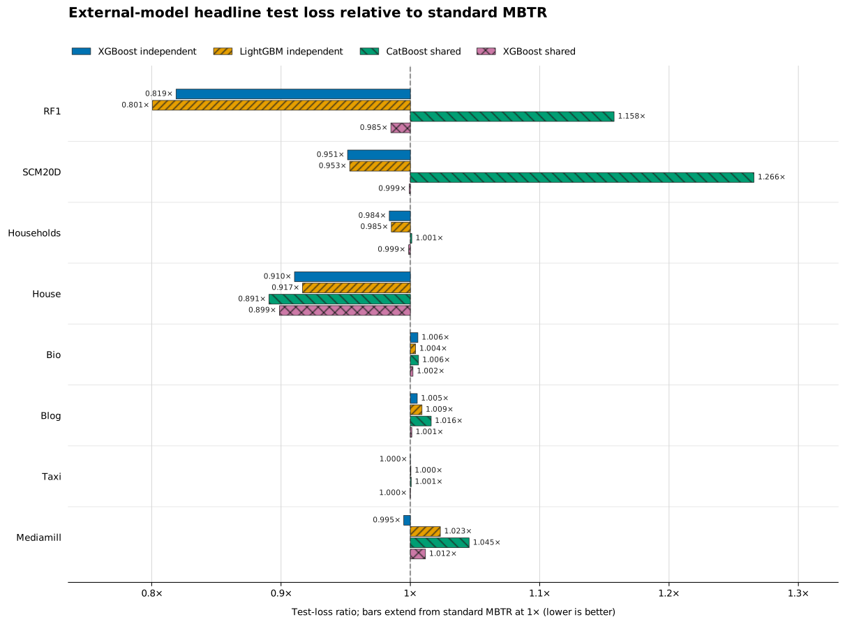
Mean paired test-loss ratio relative to standard MBTR. Every bar extends from
the 1× standard-MBTR reference; lower and farther left is better. Regression
rows use global RMSE and Mediamill uses binary cross-entropy. Annotations are
rounded, so 1.000× denotes near parity rather than necessarily exact equality.
Regression ratios use global RMSE after inverse transformation to the raw target scale, so high-variance outputs can dominate. Consult the equal-target metrics in the full report before interpreting a bar as a general multivariate improvement.
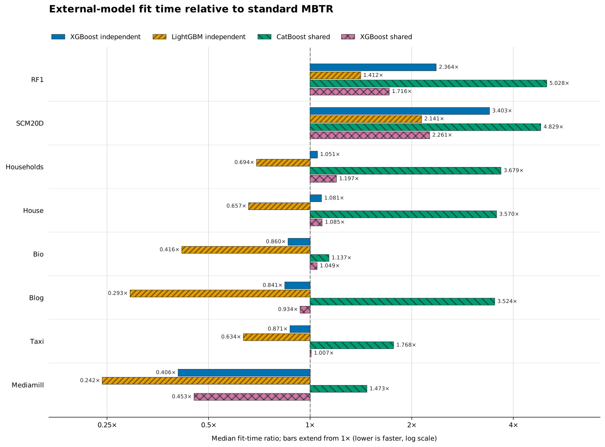
Ratio of median fitting times relative to standard MBTR. Every bar extends
from the 1× standard-MBTR reference; lower and farther left is faster. The
ratio axis is logarithmic so reciprocal ratios have equal visual distance from
the reference.
Across the four external implementations, headline loss ratios range from
0.801× to 1.266× and fit-time ratios from 0.242× to 5.028×. The
optimized standard MBTR is faster than every retained external baseline on RF1
and SCM20D and faster than CatBoost on all eight datasets; LightGBM remains
faster on six of eight. Compared with the preceding MBTR artifacts, median
standard-fit speedups range from 1.258× to 10.060×. These are fixed-setting
engineering results, not a tuned speed or accuracy ranking.
This 31 October 2026 MBTR refresh includes the eight datasets whose standard MBTR and external-baseline folds were complete. Delicious is excluded because only one of its five folds had completed. Standard MBTR was rerun after the implementation speedups. Linear-response MBTR was also rerun for the full study report, but is deliberately excluded from these figures: feature selection plus a second fit is a two-stage experiment, not a like-for-like single-model baseline. The external-model artifacts were retained from the 30 October run on the same prepared splits and one-thread protocol rather than refitted. Their quality scores therefore remain paired to the same test folds, but timing ratios between external models and MBTR compare separate local runs and are not contemporaneous wall-clock measurements.
The protocol used a 1,000-round cap, learning rate 0.05, patience 50,
validation-only iteration selection, and one final evaluation on the common
test fold. It used no method-specific hyperparameter optimization. Mediamill is
the only complete multilabel dataset in this snapshot, so it does not support
broad classification conclusions. Timings use one native thread per fit, and
equal boosting rounds do not imply equal capacity or equal physical tree
counts: an independent-output implementation may build one scalar tree per
output in a round. Several fits also reached the round cap, so neither plot
should be read as a definitive ranking of tuned algorithms.
The figures are generated from the per-fold artifacts rather than hand-entered
values. See studies/multivariate/ for the
full protocol, metric definitions, commands, and interpretation limits.
Migrating from v0.1
The compatibility class MBT remains available for one transition cycle, but
new code should use MBTRegressor.
| v0.1 | v0.2 |
|---|---|
MBT |
MBTRegressor |
n_boosts |
n_estimators |
loss_type |
objective |
n_q |
max_bins |
min_leaf |
min_samples_leaf |
lambda_weights |
l2_regularization |
lambda_leaves |
leaf_regularization |
x_lr |
response_features |
val_ratio |
explicit eval_set, or validation_fraction |
Training plots were removed from fit; use evals_result_ with your plotting
library. Quantile predictions now always expose both output and quantile axes.
Numerical results can change because v0.2 corrects split gain, minimum-leaf,
Fourier, validation, and structured-objective defects.
Documentation and reference
The full user, migration, extension, and performance guides are built from
docs/source and published at Read the Docs.
If you use MBTR in research, please cite:
Lorenzo Nespoli and Vasco Medici (2022), “Multivariate Boosted Trees and Applications to Forecasting and Control,” Journal of Machine Learning Research, 23(246):1–47. Paper
@article{JMLR:v23:21-0247,
  author  = {Lorenzo Nespoli and Vasco Medici},
  title   = {Multivariate Boosted Trees and Applications to Forecasting and Control},
  journal = {Journal of Machine Learning Research},
  year    = {2022},
  volume  = {23},
  number  = {246},
  pages   = {1--47},
  url     = {https://jmlr.org/papers/v23/21-0247.html}
}
Published applications
This curated list includes work that explicitly reports using the MBTR software or the Nespoli–Medici multivariate boosted-tree method. A citation of the foundational paper alone is not treated as evidence of use. Preprints and technical reports are labelled to distinguish them from peer-reviewed articles.
Peer-reviewed articles
- Schickele, A., Debeljak, P., Ayata, S.-D., Bittner, L., Pelletier, E., Guidi, L., and Irisson, J.-O. (2024). The genomic potential of photosynthesis in piconanoplankton is functionally redundant but taxonomically structured at a global scale. Science Advances, 10, eadl0534. doi:10.1126/sciadv.adl0534 — uses MBTR to model multivariate gene-cluster abundances from environmental climatologies.
Technical reports
- Debeljak, P., Schickele, A., Ayata, S.-D., Bittner, L., Irisson, J.-O., and Drago, F. (2022). Exploring and mapping plankton genomics data with Blue-Cloud. Zenodo. doi:10.5281/zenodo.6224852 — implements multivariate gradient boosting in R on top of the Python MBTR library.
Preprints
- Schickele, A., Savioz, H., Gruber, N., Guidi, L., Irisson, J.-O., and Vogt, M. (2025). Global pattern of nitrogen metabolism in marine prokaryotes. bioRxiv. doi:10.1101/2025.10.28.685123 (v2 posted 10 March 2026) — uses MBTR within CEPHALOPOD to project the genomic potential of nitrogen-transformation pathways.
If your work uses MBTR, please open an issue or a pull request with its DOI or permanent link and a short description of how MBTR was used.
MBTR is released under the MIT license.
1 maintainer

Metadata
1 maintainer
Release files for mbtr 0.2.0
For a detailed explanation of source distributions (sdists) and built distributions (wheels), please see the package formats documentation.
Source distribution (sdist)
| File | Size | Uploaded | Provenance | Actions |
|---|---|---|---|---|
| mbtr-0.2.0.tar.gz | 48.9 kB | Without provenance | Details for mbtr-0.2.0.tar.gz |
Built distribution (wheel)
| File | Interpreter | ABI | Platform | Actions Reset |
|---|---|---|---|---|
| mbtr-0.2.0-py3-none-any.whl | Python 3 | none | any | Details for mbtr-0.2.0-py3-none-any.whl |
Total release size: 91.4 kB
Release files / mbtr-0.2.0.tar.gz
| Download URL | mbtr-0.2.0.tar.gz |
|---|---|
| Size | 48.9 kB |
| Tags | Source |
|
SHA-256 checksum How to use checksums |
34f03eb3966d9dbcfc62bb6477d8c16b556fd75bdd5423e57ec4b59e09040c30
|
|
BLAKE2b-256 checksum How to use checksums |
29ab151746a42ccddae3ad78910d26fa31f97d495b5c22ebaf0306e6cd88361d
|
| Upload date | |
|
Uploaded using Trusted Publishing? What is trusted publishing? |
No |
| Uploaded via |
twine/7.0.0 CPython/3.13.16
|
Release files / mbtr-0.2.0-py3-none-any.whl
| Download URL | mbtr-0.2.0-py3-none-any.whl |
|---|---|
| Size | 42.5 kB |
| Tags | Python 3 |
|
SHA-256 checksum How to use checksums |
be1cd3446d122444866996e842e7fb361a898fd6c8d167b76a110a6f52eb1ef6
|
|
BLAKE2b-256 checksum How to use checksums |
ba980057599d39b5feaf281377fb18a4b66db7e08bf729dbd137d62f58d2a458
|
| Upload date | |
|
Uploaded using Trusted Publishing? What is trusted publishing? |
No |
| Uploaded via |
twine/7.0.0 CPython/3.13.16
|
Security for mbtr 0.2.0
Provenance
Provenance describes where a file came from. On PyPI, provenance is shared via attestations, which provide a verifiable record of the build or publishing details. View details, limitations and caveats.
No provenance found
None of the files in this release were uploaded with provenance metadata.
A note on package security
PyPI is a repository for distributing packages, not a service for auditing them. While third-party security researchers and our staff do their best to detect and remove malicious packages, PyPI cannot guarantee the quality, security or suitability of any given package.
To learn more about protecting yourself from malicious actors, visit our package security documentation.














