
MCPymol — talk to PyMOL



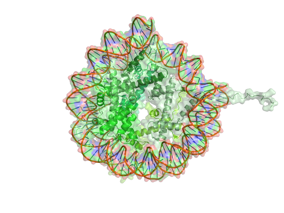
MCPymol is a Model Context Protocol server that lets you drive PyMOL with natural language. Load structures, set up analytical views, measure things, and explore proteins by talking to Claude or Gemini. The image above was made by typing "show me a nucleosome" into Claude Code. That was the whole prompt.
PyMOL is great, but its syntax is famously obscure — and despite the name, it isn't quite Python. MCPymol is for people who'd rather just look at structures.
What you get
- A vocabulary the LLM understands. Tools like
fetch_structure,ligand_view,interface_view,mutation_view,conservation_viewdo high-level setup in one call: pick the biological assembly, hide solvent, color sensibly, label the right residues, draw the right H-bonds. - Renders the model can see.
renderray-traces and hands the image straight back, so the assistant can look at what it made and fix it — rather than writing a PNG it has no way to inspect. - 87 PyMOL primitives exposed as individual tools (
show,hide,color,select,distance,align,spectrum, …) so the model can compose finer motions when the high-level tools don't quite fit. 121 tools in total, every parameter documented in the tool schema. When even that runs out,execute_pymol_commandpasses a raw PyMOL command straight through. - Predicted structures. A UniProt accession fetches from AlphaFold DB and colors by pLDDT confidence in the official palette — via
fetch_structureorfetch_alphafolddirectly. - Scene introspection.
list_objects,list_chains,list_ligandsandstructure_infolet the model check what's actually loaded before guessing,count_atomscatches a selection that matches nothing — otherwise invisible until the render comes out blank — andatom_propertiesreaches occupancy and altlocs that no per-residue view can show. - Your own files too.
load_structureopens a local PDB/mmCIF — a model you built, a docking pose, an MD frame — through the same prep and styling as a fetched entry. - Smart structure prep. Fetching a PDB code grabs the biological assembly when one exists, then runs a BFS heuristic over chain–chain contacts (
multimer_cutoff, default 8 Å) so sprawling functional multimers like the CRP pentamer or ferritin cage stay whole while crystallographic copies get dropped. Waters and crystallization additives are hidden automatically. - Two-process bridge. PyMOL's GUI has its own Python; MCPymol works by running a tiny TCP listener inside PyMOL plus a separate FastMCP server outside it.
How it talks
┌──────────────┐   MCP / stdio    ┌────────────────┐  JSON over TCP  ┌──────────────┐
│ Claude /     │ ───────────────▶ │ mcpymol server │ ◀────:9876────▶ │ PyMOL GUI    │
│ Gemini CLI   │                  │   (FastMCP)    │                 │  (plugin.py) │
└──────────────┘                  └────────────────┘                 └──────────────┘
The plugin half runs inside PyMOL and dispatches to pymol.cmd. The bridge half is what the MCP client launches. They talk over a local TCP socket because PyMOL's GUI ships its own Python interpreter, which cannot import the packages the MCP server needs — so the two halves cannot live in one process.
Both halves must run on the same machine: several tools hand files between them through the filesystem.
Try it
"Fetch ubiquitin (1ubq) and show it as a cartoon, then show me the render." "Color the alpha helices red and the beta sheets blue." "What ligands are in 1HSG?" "Show the binding pocket around MK1 in 1HSG." "Highlight mutations E6V, K16E, and V67F in hemoglobin (4HHB)." "Run a Poisson-Boltzmann electrostatics calculation on 1LYZ." "Get the AlphaFold model for P69905 and tell me how confident it is." "Superpose 1AKE onto 4AKE and show me where adenylate kinase moves." "Make me a turntable animation of the nucleosome."
Tip: if the model isn't sure what's loaded, ask it to list the objects — it'll call list_objects and ground itself before guessing names.
What can I ask?
Organised by the question, not the tool.
| Question | Tool |
|---|---|
| What is this structure — resolution, method, organism? | structure_info |
| What's the sequence, and how does it map to the residue numbering? | get_sequence |
| What's loaded / what chains / what ligands? | list_objects, list_chains, list_ligands |
| Can I open my own file rather than a PDB code? | load_structure |
| What are this atom's occupancy / altloc / B-factor? | atom_properties |
| What holds this ligand in its pocket, and how tightly? | contact_report, then ligand_view to see it |
| How big is this interface, and which residues matter? | interface_report, then interface_view |
| Where do these two structures differ? | superposition_view |
| How far apart / what angle / how much surface? | distance, angle, dihedral, sasa, rms_cur |
| Which parts are conserved? Flexible? Confident? | conservation_view, bfactor_view, plddt_view |
| What does it look like? | render — returns the image, so the model can see it |
| Can I keep this scene? | save_session / load_session |
| Can I print it? | print_ribbon_view + print_export |
The pattern that works best: report first, then draw. contact_report tells
you Asp30 makes a salt bridge at 2.7 Å; ligand_view then shows you where it
sits. Asking only for the picture gets you a picture you have to interpret
yourself.
Requirements
- PyMOL — the open-source build is what this is developed against (
brew install pymolon macOS,apt-get install pymolon Debian/Ubuntu). The Schrödinger incentive build works too. MCPymol drives a PyMOL you already have; it does not install or bundle one. - Python 3.10+ for the bridge. This is separate from the Python inside PyMOL, which MCPymol never imports into.
- An MCP client — Claude Code, Claude Desktop, or Gemini CLI.
Optional, per feature:
| For | You also need |
|---|---|
poisson_boltzmann_view |
apbs and pdb2pqr on PATH |
print_export, print_ribbon_view |
the print extra — install it the way you installed MCPymol, e.g. uv tool install 'mcpymol[print]' (see 3D Printing Export) |
conservation_view |
network access to an MMseqs2 server (ColabFold's public API by default) |
fetch_structure, structure_info |
network access to the RCSB |
Installation
There are two halves to wire up: the native plugin (runs inside PyMOL) and the MCP bridge (runs outside, and is what your AI assistant launches). Both come from the same package.
1. Install MCPymol
uv tool install mcpymol
pipx install mcpymol works the same way. There is no need to clone the
repository unless you intend to work on MCPymol itself.
Check it landed somewhere your shell can see:
which mcpymol # if this prints nothing, run: uv tool update-shell
Note the full path it prints — you will want it in step 3. uv and pipx
install into ~/.local/bin, which is not on everyone's PATH, and an MCP client
started by the OS rather than from your shell does not inherit your PATH at
all. Wiring the assistant to a bare mcpymol when it is not on PATH fails at
launch with spawn mcpymol ENOENT, not at install time.
Why not
uvx mcpymol?uvxruns the bridge perfectly well, but it is the wrong tool for step 2: it unpacks the package into~/.cache/uv, and the plugin has to be loaded by absolute path, so the line written into your PyMOL startup file would point into a cache thatuv cache cleanreclaims.uv tool installputs it somewhere permanent — and lets both halves come from one installation, so the bridge and the plugin cannot drift apart.
2. Start the native plugin
The plugin runs inside PyMOL, which has its own Python interpreter — it cannot import the installed package, so it is loaded from a file path. Let MCPymol find that path for you:
mcpymol --install-plugin
That adds a small managed block to ~/.pymolrc.py, so PyMOL loads the plugin
on every launch. Restart PyMOL and you should see:
MCPymol Native Plugin listening on 127.0.0.1:9876
Re-run it after upgrading MCPymol — the block embeds a path into one
installation and is rewritten, not duplicated. mcpymol --uninstall-plugin
removes it and leaves the rest of your .pymolrc.py alone.
If you would rather wire it up yourself, mcpymol --plugin-path prints the
path, and you can run it from the PyMOL command line or add your own line to
~/.pymolrc.py.
Changing the port. Set MCPYMOL_PORT before launching both PyMOL and
the bridge — see Configuration.
3. Register the bridge with your AI assistant
Pick one. Use the full path from which mcpymol — it is the same
installation the plugin came from, and a bare mcpymol only works if that
directory is on the PATH of whatever launches the client.
Claude Code CLI
claude mcp add mcpymol -- "$(which mcpymol)"
Start a new Claude Code session.
Claude Desktop
Add to claude_desktop_config.json:
{
  "mcpServers": {
    "mcpymol": {
      "command": "/absolute/path/to/mcpymol"
    }
  }
}
The absolute path is not optional here: Claude Desktop is launched by the OS rather than from your shell, so it never inherits your PATH. Restart Claude Desktop afterwards.
Gemini CLI
gemini mcp add mcpymol "$(which mcpymol)"
gemini mcp refresh
Without installing — uvx
To run the bridge without installing anything, point your assistant at
uvx mcpymol:
claude mcp add mcpymol -- uvx mcpymol
You still need the plugin, and step 2's command is not available to you —
nothing was installed. Run it through uvx instead:
uvx mcpymol --install-plugin
That writes a path into ~/.cache/uv (see the note in step 1), so uv cache clean or a uvx upgrade will break it and you will have to re-run it. uvx
also resolves the newest release on each launch, so the bridge can drift ahead
of the plugin. This path trades a permanent install for maintenance; if that
sounds worse than installing, install.
Restricted environments — no uv
If uv is blocked by your org's security policy, use a standard venv. On Linux you may need sudo apt-get install python3-venv pymol first.
python3 -m venv ~/.venvs/mcpymol
~/.venvs/mcpymol/bin/pip install --upgrade pip
~/.venvs/mcpymol/bin/pip install mcpymol
~/.venvs/mcpymol/bin/mcpymol --install-plugin

# Point the assistant directly at the venv binary
claude mcp add mcpymol ~/.venvs/mcpymol/bin/mcpymol
# or
gemini mcp add mcpymol ~/.venvs/mcpymol/bin/mcpymol
If your network blocks PyPI, install from your internal mirror with pip install --index-url ....
Upgrading
Upgrade the way you installed — uv tool upgrade mcpymol, pipx upgrade mcpymol, or <venv>/bin/pip install --upgrade mcpymol. Then restart
PyMOL and reconnect the MCP server in your client (/mcp in Claude Code).
Both halves have to move together, and neither moves on its own. The plugin is loaded into PyMOL's memory at startup, and the bridge is a process your MCP client launched — upgrading the package on disk changes neither until each is restarted. PyMOL will happily keep running the plugin it loaded days ago against a freshly upgraded bridge.
You do not normally need to re-run --install-plugin: uv tool, pipx and
a venv all upgrade the package in place, so the path in ~/.pymolrc.py still
points at the right file. Re-run it if you move the installation — switching
install method, rebuilding the venv, or using the uvx path, whose cache
directory does change.
A mismatched pair fails in a way that reads like a bug in a tool rather than a stale process: calls that should work report unknown actions, or a tool fixed in the release you just installed keeps misbehaving.
Working on MCPymol itself
For development, clone the repo and run from the checkout — this is the only path that needs a clone:
git clone https://github.com/chemrich/MCPymol.git
cd MCPymol
uv sync
uv run mcpymol --install-plugin
claude mcp add mcpymol -- uv --directory /absolute/path/to/MCPymol run mcpymol
See CONTRIBUTING.md.
Configuration
Everything is optional; the defaults are what the tools are tuned for. Set them before launching PyMOL and the bridge.
| Variable | Default | What it does |
|---|---|---|
MCPYMOL_PORT |
9876 |
Bridge ↔ plugin TCP port. Must match on both sides. |
MCPYMOL_RECV_TIMEOUT |
30 s |
How long the plugin waits for one complete request before answering with an error. Bounds how long a stalled client can hold the single-threaded accept loop. |
MCPYMOL_MAX_REQUEST_BYTES |
8388608 |
Largest single request the plugin will accept. |
MCPYMOL_SLOW_OP_TIMEOUT |
600 s |
Socket budget for operations that legitimately take minutes — ray, png, save, mpng, draw. |
MCPYMOL_MAX_IMAGE_BYTES |
5000000 |
Above this, render returns the file path instead of inlining the image. |
MCPYMOL_PB_TIMEOUT |
600 s |
Wall-clock ceiling on the external apbs / pdb2pqr processes. |
MCPYMOL_MMSEQS_URL |
ColabFold public API | MMseqs2 server for conservation_view. Point at an internal one to avoid the public queue. |
MCPYMOL_ALPHAFOLD_API_URL |
AlphaFold DB prediction API | Where fetch_alphafold asks which model file is current. |
MCPYMOL_ALPHAFOLD_URL |
AlphaFold DB files | Legacy filename template, used only when you pin model_version explicitly. |
MCPYMOL_RCSB_URL |
RCSB data API | Base URL for the metadata structure_info reports. |
MCPYMOL_PORT=9867 open -a PyMOL       # macOS
MCPYMOL_PORT=9867 mcpymol             # bridge
Troubleshooting
| Symptom | Likely cause | Fix |
|---|---|---|
| Every tool returns "Socket connection failed. Is the PyMOL plugin running?" | Plugin not loaded in PyMOL | run /path/to/plugin.py inside PyMOL, or add it to ~/.pymolrc.py |
| "Address already in use" on plugin start | A previous PyMOL session left the port open, or another app uses 9876 | Quit lingering PyMOL processes, or set MCPYMOL_PORT=9867 on both sides |
Long get_fastastr / get_chains calls fail with a JSON parse error |
You're on a pre-2026-05 version of MCPymol that capped recv() at 8 KB | Upgrade — the bridge now drains the response in full |
conservation_view is slow |
First call hits the ColabFold MMseqs2 API (30 s–few min); subsequent calls for the same sequence hit a local cache | If you have an internal MMseqs2 server, set MCPYMOL_MMSEQS_URL |
poisson_boltzmann_view fails |
apbs or pdb2pqr missing |
brew install brewsci/bio/apbs and pip install pdb2pqr |
| A tool reports a file "did not appear" | PyMOL and the bridge are on different machines — they exchange files through the filesystem | Run both on the same host |
render returns a size message instead of an image |
The PNG exceeded the inline limit; base64 inflates it by a third | Ask for a smaller width/height, or raise MCPYMOL_MAX_IMAGE_BYTES |
fetch_structure/fetch_alphafold says "No AlphaFold model" |
The accession is valid but AlphaFold DB has no model at that version | Try another model_version, or check the accession |
| A view comes out blank | The selection matched no atoms | count_atoms on the selection before building the scene |
| A long operation returns "Socket connection failed: timed out" | Something slower than its budget | Raise MCPYMOL_SLOW_OP_TIMEOUT (renders, saves) or MCPYMOL_PB_TIMEOUT (APBS) |
| A tool reports an unknown action, or a bug you just upgraded past is still there | PyMOL is still running the plugin it loaded at startup, from before the upgrade | Restart PyMOL, then reconnect the server in your client (/mcp in Claude Code) — see Upgrading |
| New tools don't show up after an upgrade | The MCP client is still running the previous bridge process | Reconnect the server in your client, or start a new session |
| A fetch reports success but nothing is loaded | Pre-v1.4.0 behaviour: cmd.fetch doesn't raise on a failed download |
Upgrade — fetches now verify atoms arrived and say so plainly, and no longer clear the session on failure |
render says the image is "a single flat colour" |
The camera is pointed at nothing, or the session is wedged after heavy use | zoom on the object, or restart PyMOL if zoom stops responding |
Tests
uv run pytest
555 tests run by default. They mock the socket layer and PyMOL's cmd module, so they need neither PyMOL nor a network, and cover the socket payloads, the bridge framing, the conservation pipeline (A3M parsing, Shannon entropy, MMseqs2 mocking, MSA→B-factor mapping), the mesh-repair paths, and every view. tests/test_bridge_roundtrip.py additionally runs the real bridge against the real plugin listener over TCP on an ephemeral port, so the wire format is checked against itself rather than against a mock.
The two opt-in suites
A further 122 tests are deselected by default, because they need things CI does not have. Both are worth running before a release tag:
uv run pytest -m live      # needs a running PyMOL with the plugin loaded
uv run pytest -m network   # hits real external APIs
-m liveclears the PyMOL session it connects to. It drives your actual PyMOL. Don't run it against a session you care about.
-m live exists because a mocked suite asserts the payload we send, which can never tell you whether PyMOL will accept it — and that gap is where every wiring bug has lived: tools calling cmd functions that don't exist, arguments bound in the wrong order, renders that come back blank. It calls every registered tool once and asserts only that each is wired (the action resolves, the arguments bind), not that it succeeds, since many tools error honestly without the right context. New tools are swept automatically. It skips cleanly when no PyMOL is listening, and detects a wedged session rather than reporting a hundred confusing failures.
Treat a green default run as necessary, not sufficient.
Layout
| Module | Responsibility |
|---|---|
mcpymol/app.py |
the shared FastMCP application |
mcpymol/bridge.py |
socket protocol to the in-PyMOL plugin |
mcpymol/structures.py |
fetching/loading structures, sessions, introspection |
mcpymol/primitives.py |
one thin tool per pymol.cmd function |
mcpymol/views.py |
the *_view scene presets |
mcpymol/style.py |
scene conventions shared across the presets |
mcpymol/rendering.py |
render, turntable |
mcpymol/comparison.py |
superposition_view |
mcpymol/conservation.py |
MSA + Shannon entropy |
mcpymol/analysis.py |
contact_report, interface_report |
mcpymol/pdbtext.py |
parsing the PDB records PyMOL hands back as text |
mcpymol/printing.py |
watertight STL export |
mcpymol/cli.py |
--install-plugin, --plugin-path, --uninstall-plugin |
mcpymol/plugin.py |
the half that runs inside PyMOL |
mcpymol/server.py is the entry point and re-exports everything, so from mcpymol.server import ligand_view still works.
The view library
These are the high-level visualization tools. Each does its own setup — coloring, transparency, H-bonds, labels — in one prompt.
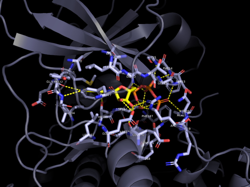
ligand_view — binding site
Pocket residues (within 5 Å of the ligand) as element-colored sticks with CA labels, ligand as yellow sticks, H-bonds as yellow dashes, protein as a translucent cartoon.
Show me the ATP binding site in 1ATP
interface_view — protein–protein interface
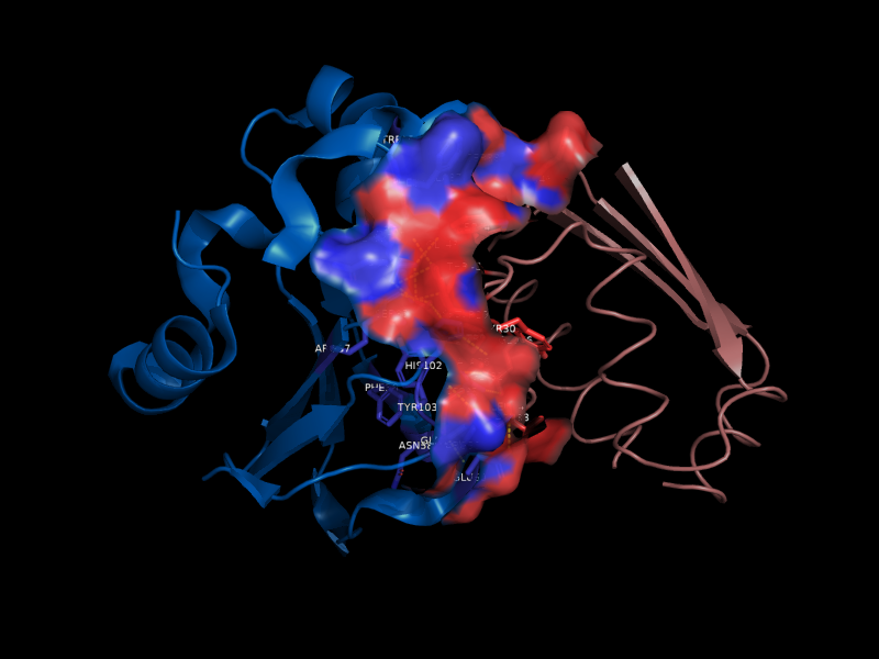
Chain A marine, chain B salmon. Interface residues (within 4 Å of the partner) as solid surface patches with sidechain sticks and CA labels. Cross-chain H-bonds as yellow dashes.
Show the interface between chain A and chain D in 1BRS
putty_view — B-factor flexibility
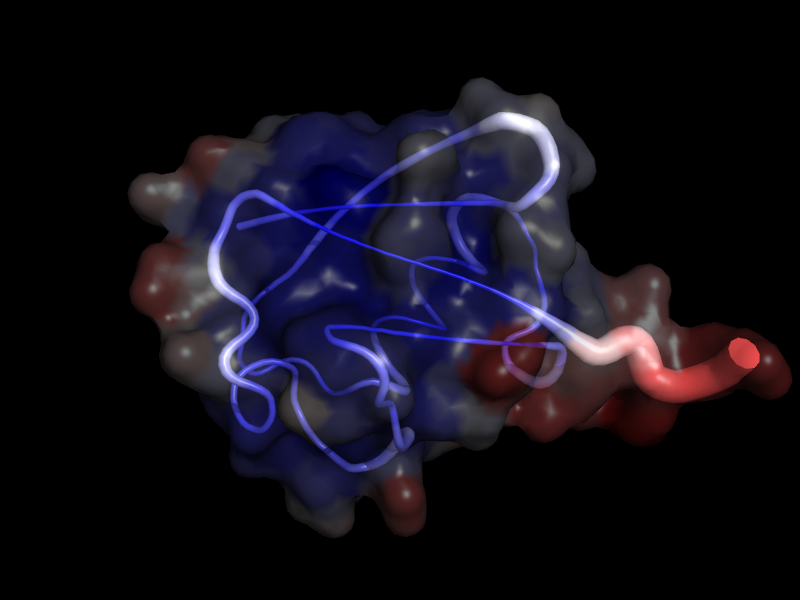
Tube radius and color scale with B-factor: blue/thin = rigid, red/thick = flexible. A 70%-transparent surface adds shape context.
Show the B-factor flexibility of 1UBQ as a putty view
bfactor_view — B-factor flexibility, plain cartoon
The same color story as putty_view (blue → red on B-factor) but on a plain cartoon. Cheaper, cleaner in figures where you don't want the putty distortion.
Color 1UBQ by B-factor
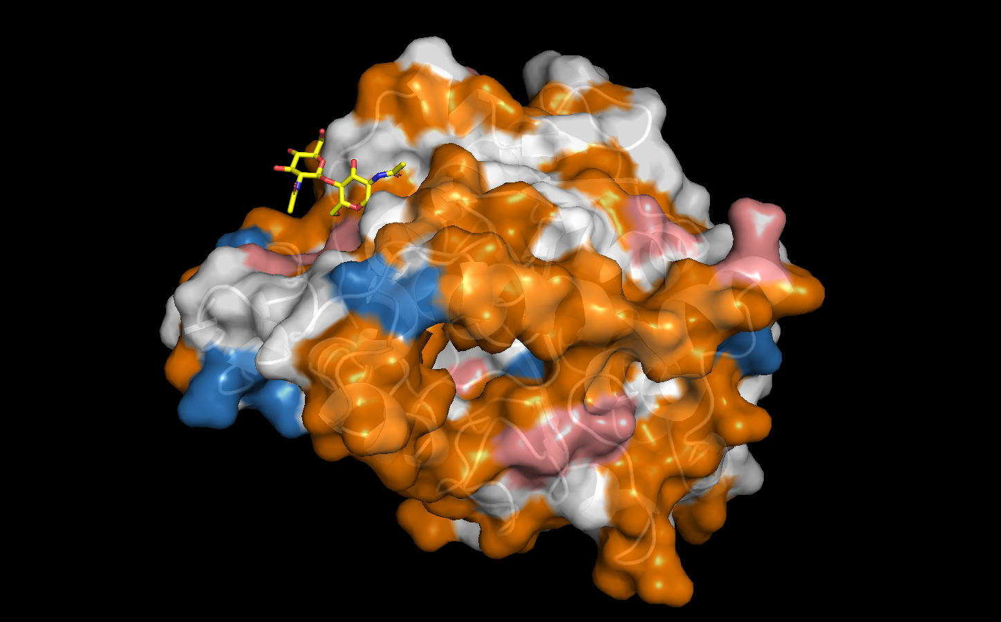
hydrophobic_surface_view — surface chemistry
Surface colored by amino-acid chemistry: orange = hydrophobic, white = polar, sky blue = positive, salmon = negative. Useful for spotting hydrophobic patches, membrane belts, and charge complementarity.
Show the hydrophobic surface of 1TCA
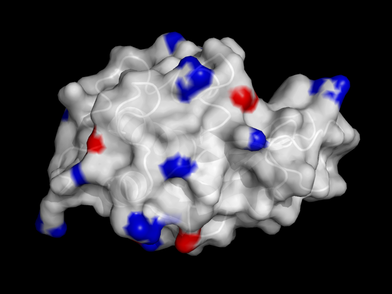
electrostatic_view — approximate electrostatics
Red→white→blue surface coloring driven by per-residue pKa-weighted partial charges. Two modes: atomic (charges on the actual charge-center atoms — localized, natural falloff) and residue (uniform across charged residues — saturated patches).
Show the electrostatic surface of 1LYZ
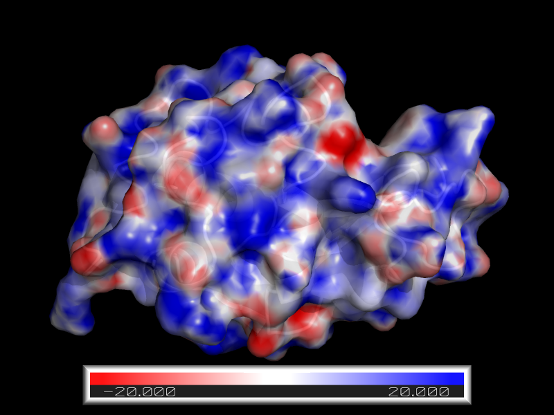
poisson_boltzmann_view — true PB electrostatics
Full Poisson-Boltzmann potential via APBS and PDB2PQR, mapped onto the surface at ±20 kT/e. Physically correct, accounts for solvent screening and ionic strength.
Prerequisites (must be on
PATH):brew install brewsci/bio/apbs pip install pdb2pqr
Run a Poisson-Boltzmann electrostatics calculation on 1LYZ
conservation_view — evolutionary conservation
Pipeline: extract the chain's sequence → submit to MMseqs2 (ColabFold public API by default; override with MCPYMOL_MMSEQS_URL) → parse the A3M alignment → compute per-position Shannon entropy → map onto B-factor and color via cyan_white_magenta spectrum.
Magenta = conserved, white = moderate, cyan = variable. First call takes 30 s – few minutes depending on sequence length; results are cached in memory by sequence, so re-running on the same protein (or changing only the color scale) is instant.
Color lysozyme (1LYZ) by conservation
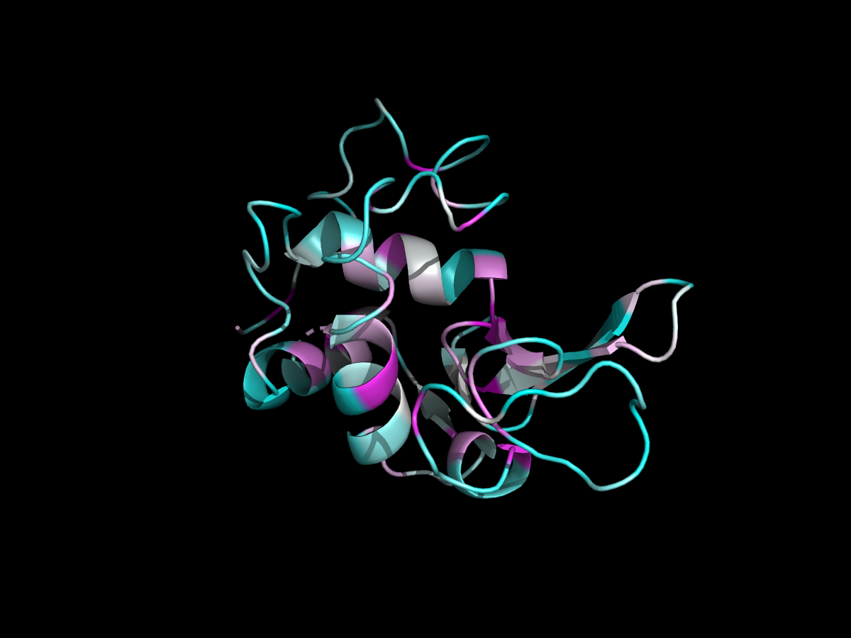
Lysozyme against 5,507 homologues. The variable surface loops go cyan while the core and the substrate-binding cleft stay magenta — conservation tracking function, which is the whole reason to compute it.
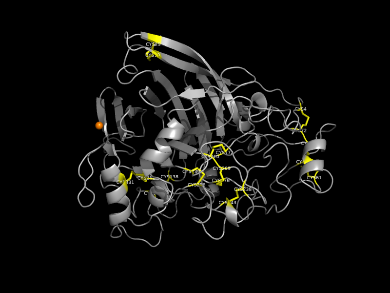
crosslink_view — disulfides & metal coordination
CYS sidechains and disulfide bonds in yellow, metal coordination bonds in orange, the rest of the protein as a thin grey cartoon.
Show the disulfide bonds in 1CEL
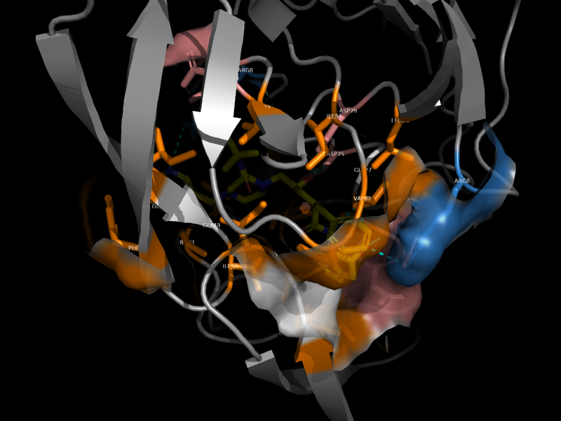
pocket_view — binding pocket surface
The pocket cavity (residues within 5 Å of the ligand) as a semi-transparent surface colored by chemistry. Sticks for the pocket sidechains, yellow sticks for the ligand, cyan dashes for H-bonds.
Show the binding pocket around MK1 in 1HSG
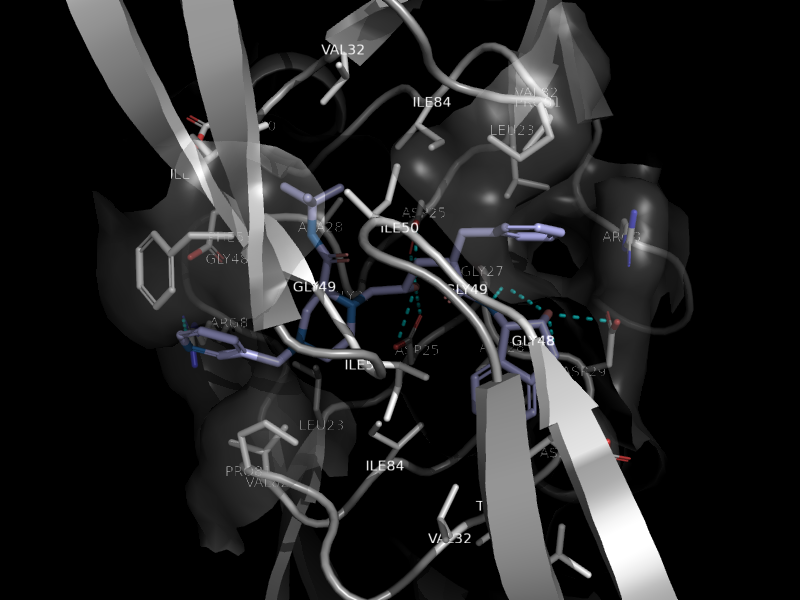
pharmacophore_view — ligand pharmacophore features
The ligand colored by pharmacophore type: violet = aromatic ring carbon, yellow = aliphatic carbon, sky blue = N (donor/acceptor), salmon = O (acceptor), gold = S, pale green = halogen. Interacting residue sticks with CA labels, cyan dashes for H-bonds.
Show the pharmacophore features of MK1 in 1HSG
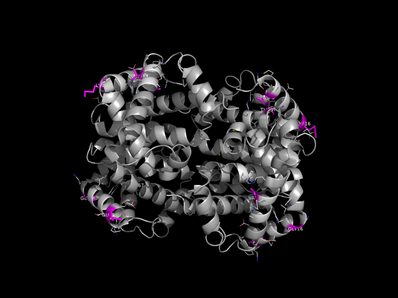
mutation_view — mutation hotspots
Grey cartoon, mutated sidechains as magenta sticks with white CA labels, neighboring residues (within 4 Å) as thin element-colored sticks for packing context. Standard A123G notation; optional chain prefix A:A123G.
Highlight mutations E6V, K16E, and V67F in hemoglobin (4HHB)
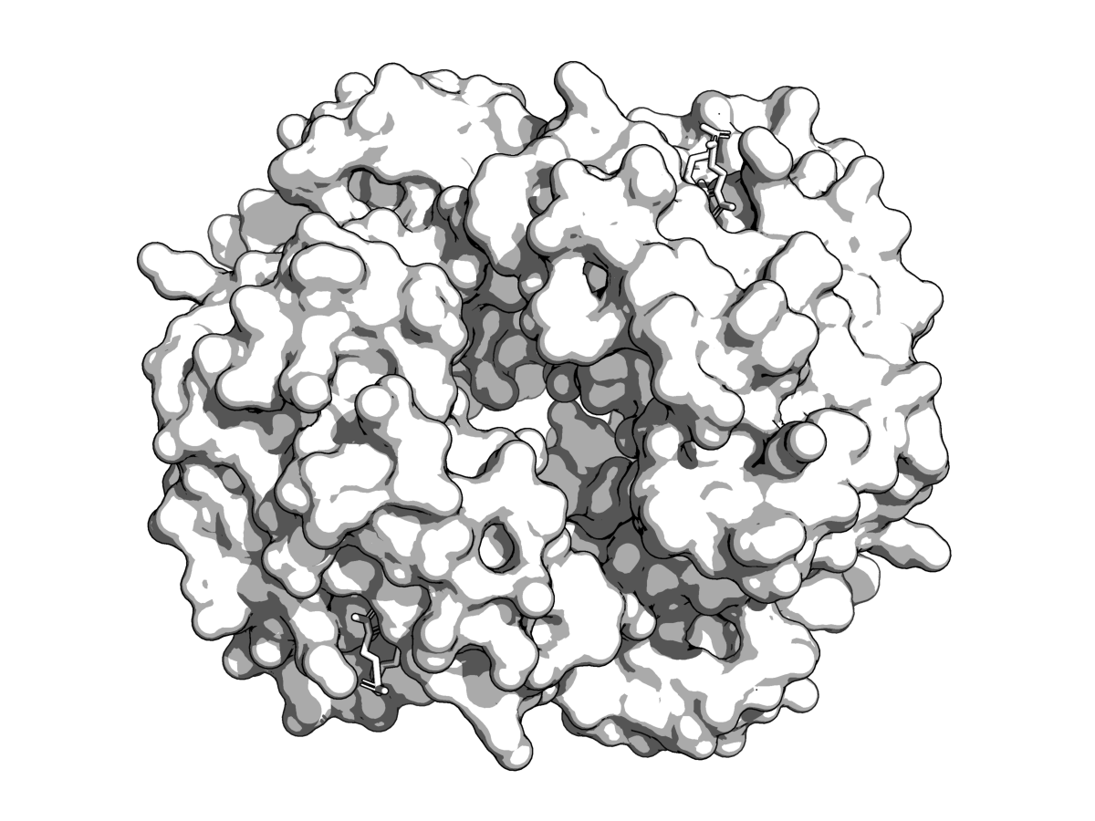
textbook_view — cel-shaded illustration
White cartoon + surface with heavy ray-trace contours. The cel-shaded look kicks in after you run ray (or ask the model to render).
Make 4HHB look like a textbook illustration
cinematic_view — fog and shadows
Depth-cueing + fog + soft shadows on a black background. Best on big assemblies — ribosomes, capsids, nucleosomes — where you want a sense of scale. Run ray for the full effect.
Give me a cinematic view of GroEL
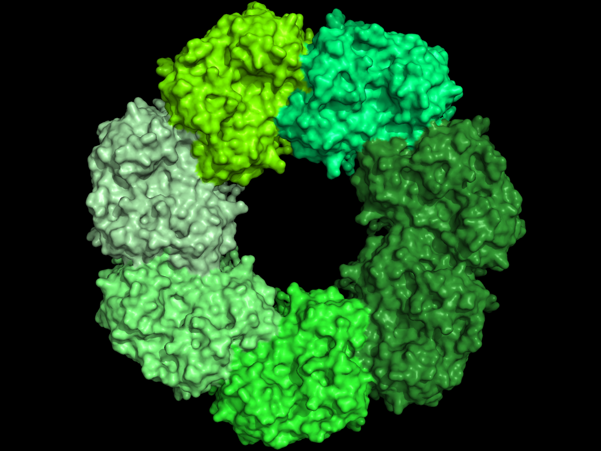
Depth cueing needs scale to pay off — this is one GroEL ring down its seven-fold axis. On a small globular protein the effect is mostly lost.
pointillist_view — starfield surface
Replaces the surface with a dense dot cloud; ligands become bright yellow stars. More art than analysis.
plddt_view — AlphaFold confidence
Colors a predicted model by pLDDT in AlphaFold's official palette: dark blue >90 (very high), light blue 70–90 (confident), yellow 50–70 (low), orange <50 (very low). Reports the breakdown, e.g. "very high: 62%, confident: 21%, …".
pLDDT is stored in the B-factor column, which is why bfactor_view and putty_view render these models backwards — they read low B as rigid, whereas low pLDDT means the model doesn't know. plddt_view warns if the B-factors don't look like pLDDT at all.
Get the AlphaFold model for P0DTC2
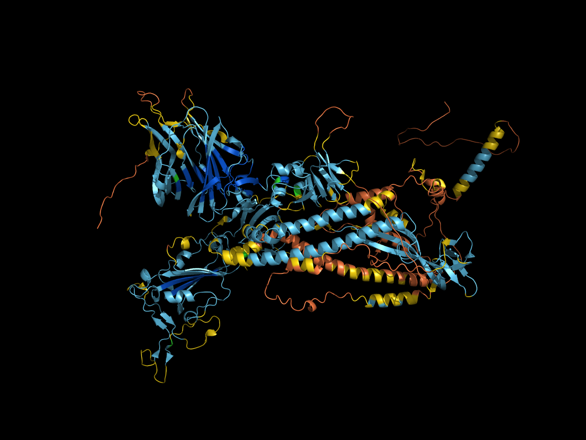
Mean pLDDT 67.1 across 1273 residues — 7% very high, 49% confident, 20% low, 24% very low. The orange tails are the point: AlphaFold is telling you it does not know where they go, and no amount of rendering makes that a structure.
superposition_view — where two structures differ
Superposes mobile onto target, then colors the mobile structure by how far each residue's CA actually moved: blue = unchanged, red = most shifted. The target stays as a grey reference. Reports the RMSD, the mean and max shift, and names the worst-shifted residues.
An RMSD alone tells you a structure moved; this tells you where.
Superpose 4AKE onto 1AKE and show me where it moves
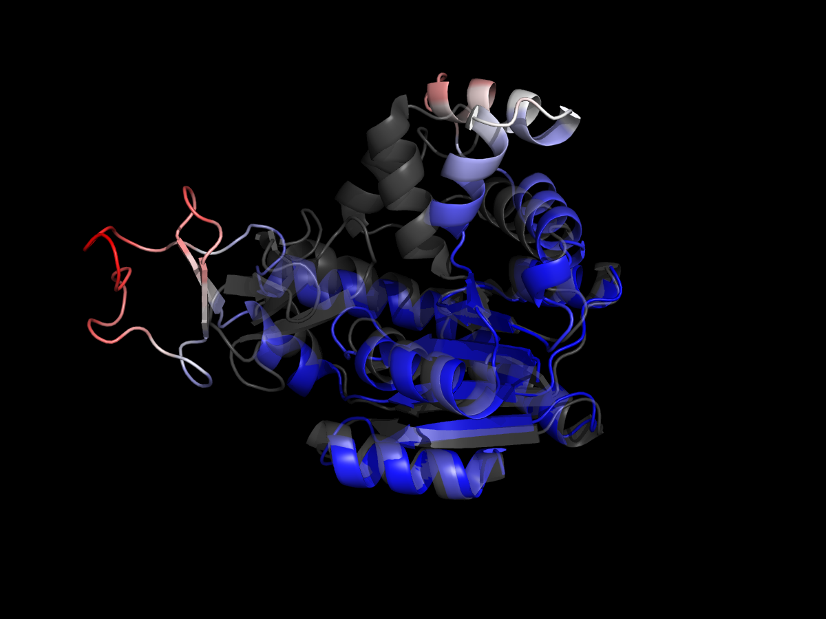
Adenylate kinase, open against closed: the core fits at 2.07 Å RMSD while residues 145–152 move up to 24 Å. That is the LID domain closing over the substrate, and it is the whole reason to colour by deviation rather than quote one number.
Both structures have to be loaded at once, and fetch_structure clears the
session by default — fetch the second with replace=False. Compare single
chains when the entries are multimers: superposing one dimer onto another fits
the assembly rather than the fold, which reports 18.5 Å for this same pair.
Analysis — answers with numbers
The view presets draw interactions; these report them. Both matter, and they compose: run the report to get the numbers for your figure legend, run the view to make the figure.
contact_report — what touches what
Lists contacting residue pairs closest first, with the minimum heavy-atom distance, how many atoms are involved, and a classification: salt bridge, hydrogen bond, hydrophobic, polar contact, or π-stacking (parallel vs T-shaped from the interplanar angle).
contact_report("1hsg and resn MK1", "1hsg and polymer")
Criteria are heavy-atom distances — salt bridge ≤ 4.0 Å between charged sidechain tips, H-bond ≤ 3.5 Å between N/O pairs, hydrophobic ≤ 4.5 Å between C/S, ring centroids ≤ 5.5 Å — because crystal structures usually have no hydrogens. A reported hydrogen bond is therefore a donor–acceptor pair with plausible geometry, not one verified against a hydrogen position.
Ring perception needs bond orders, which a PDB dump doesn't carry, so aromatics are detected for the standard aromatic amino acids only; ligand rings show up as hydrophobic contacts rather than being mis-called as stacking.
What holds MK1 in the HIV protease pocket?
26 residue pairs in contact within 4.0 A between '1hsg and resn MK1' and '1hsg and polymer':

  B/MK1902     -- B/ASP25       2.63 A  hydrogen bond, polar contact, contact (8 atom contacts)
  B/MK1902     -- A/ASP25       2.77 A  hydrogen bond, contact (8 atom contacts)
  B/MK1902     -- B/GLY27       3.03 A  hydrogen bond, polar contact, contact (8 atom contacts)
  B/MK1902     -- B/ASP29       3.06 A  hydrogen bond, polar contact, contact (6 atom contacts)
  B/MK1902     -- A/GLY48       3.15 A  hydrophobic, contact (6 atom contacts)
  B/MK1902     -- B/VAL32       3.32 A  hydrophobic (2 atom contacts)
  ... and 20 more pairs (raise max_pairs to see).

Interaction types across all pairs: 20 hydrophobic, 14 contact, 5 hydrogen bond, 4 polar contact.
Both copies of the catalytic Asp25 — one from each chain of the protease dimer —
hydrogen bond the inhibitor at 2.63 and 2.77 Å. That is the interaction the drug
was designed to make, read straight off the structure. It is the same pocket the
ligand_view image above shows; the picture and the numbers are two views of one
question.
interface_report — how big is this interface
Buried surface area from ΔSASA (free minus bound), the per-side figure papers quote, a ranking of residues by how much surface each buries, and a breakdown by residue chemistry.
It also interprets the number: under ~400 Ų per side is usually crystal packing rather than a biological interface; over ~1000 Ų is a substantial, likely specific association. Guidance from PDB-wide surveys, not a verdict.
How big is the barnase–barstar interface in 1BRS?
Interface between chains A and D of 1brs:
  Buried surface area: 777 A^2 per side (1,553 A^2 total).
  That is a typical size for a specific but transient protein-protein interface.
  Interface residues: 22 in chain A, 19 in chain D.
  Composition by buried area: 41% charged, 32% polar, 28% hydrophobic.
  Chain A hot spots: ARG59 (154 A^2), HIS102 (107 A^2), ARG83 (78 A^2), GLU60 (69 A^2), ...
  Chain D hot spots: ASP35 (120 A^2), TYR29 (97 A^2), ASP39 (86 A^2), TRP44 (75 A^2), ...
Barnase–barstar is the textbook electrostatically-driven interface, and the numbers say so unprompted: 41% of the buried area is charged, and the hot spots it ranks — Arg59/His102 on barnase, Asp35/Asp39/Trp44 on barstar — are the residues the mutagenesis literature identifies.
structure_info and get_sequence — what am I looking at
structure_info combines what PyMOL knows (chains, counts, ligands, states,
space group) with RCSB entry metadata (title, method, resolution, release date,
source organism), and flags a probable AlphaFold model when the B-factor column
looks like pLDDT.
1hsg — CRYSTAL STRUCTURE AT 1.9 ANGSTROMS RESOLUTION OF HUMAN IMMUNODEFICIENCY
VIRUS (HIV) II PROTEASE COMPLEXED WITH L-735,524, AN ORALLY BIOAVAILABLE
INHIBITOR OF THE HIV PROTEASES
  X-RAY DIFFRACTION, 2.00 A resolution, released 1996-04-03
  Source: Human immunodeficiency virus 1
  1,686 atoms, 198 residues, 127 waters
  Chains (2): A, B
  Ligands in '1hsg': MK1
  Space group P 21 21 2, cell 59.6 x 87.1 x 46.7 A
atom_properties reads properties that live on individual atoms rather than
residues or objects — occupancy, alternate conformations, per-atom B-factor,
formal charge. Nothing else reaches them: the PyMOL call that exposes them
returns an object that cannot cross the bridge, so the plugin flattens it on
the way out.
2 atoms in '1hsg and resi 25':

  chain  resi  resn  name  b      q
  A      25    ASP   OD1   18.42  1.00
  A      25    ASP   OD2   21.07  0.50
That 0.50 is the tool's reason to exist: a sidechain modelled in two conformations, invisible to every per-residue view.
get_sequence returns FASTA — plus the two things the sequence alone hides and
that routinely cause mistakes: the numbering offset (PDB numbering rarely
starts at 1, so "residue 50" in a paper and position 50 in the sequence are
usually different residues) and chain breaks where loops went unmodelled.
Rendering and sessions
render — see what you made
Ray-traces the current scene and returns the image as MCP image content, so the model can actually look at it and iterate. This is the tool to use instead of ray + png, which only leave a file behind.
Defaults to 1000×750 — the image is inlined into the conversation, and base64 inflates it by a third. Above 5 MB (MCPYMOL_MAX_IMAGE_BYTES) it returns the path instead, and keeps the file there even if you did not pass a filename, so a render that took minutes is not thrown away for being too big to show.
Every render is ray-traced, and ray_trace=False does not change that: PyMOL's fast unshaded frame grab needs its GUI thread, which the plugin does not run on, so that path wrote blank images. The flag is accepted and ignored, with a note in the reply, rather than silently handing back a blank PNG. To make a render cheaper, ask for a smaller width/height. render also detects the two ways an image comes back empty — a single flat colour, or nothing written at all — and says so instead of returning a black square.
turntable — 360° animation
Writes a numbered PNG sequence spinning the camera a full turn, plus the ffmpeg command to assemble it. Defaults to 36 frames (10° apart) at 800×600.
Every frame is ray-traced, for the same reason render is — the unshaded OpenGL path silently produced blank frames over this bridge. That makes it slow: 36 frames of a large assembly can take an hour, so start with a low frames count and a small width/height before committing to a long run.
Make me a turntable animation of 1AOI
save_session / load_session — keep a scene
.pse round-trips the entire session: every object, selection, representation, color, scene and the camera. Save before experimenting with a scene that took effort to build. load_session(merge=True) adds a saved scene to the current one rather than replacing it.
🖨️ 3D Printing Export
The print_export tool turns a structure into watertight STL files ready for
multi-colour 3D printing. PyMOL's open-source build can't write STL and its OBJ
exporter dumps the whole visible scene as non-manifold surface soup —
print_export works around all of that: it isolates each colour group, exports
it, and rebuilds a single watertight, manifold solid per group. Every group
stays in the same coordinate frame, so a slicer can load them as aligned
multi-material parts.
This tool needs the optional print extra (trimesh, pymeshlab, scipy,
scikit-image, networkx):
Install it into the same environment MCPymol is already in — a bare
pip install picks whatever pip is first on your PATH, which is usually a
different interpreter entirely, and leaves print_export still reporting the
dependencies missing:
uv tool install 'mcpymol[print]'                   # if you used uv tool
pipx install --force 'mcpymol[print]'              # if you used pipx
~/.venvs/mcpymol/bin/pip install 'mcpymol[print]'  # if you used a venv
uv sync --extra print                              # from a checkout
Re-running over an existing install is fine — it adds the extra in place.
Export T7 RNA polymerase (1MSW) for 3D printing with the protein and the
nucleic acid as separate colours
This produces one STL per group (e.g. 1MSW_protein.stl,
1MSW_nucleic.stl). method="auto" (default) picks the cheapest path that
works: compact structures (e.g. a GFP barrel) often export already-watertight,
so it does a light cleanup — keeping the largest body and dropping tiny
internal cavity shells — rather than Poisson, which can degrade an
already-closed surface. Otherwise it falls back to Poisson, then voxel.
method="poisson" forces detail-preserving reconstruction (best for bulky
chains); method="voxel" is robust for thin nucleic acids and slightly
thickens fragile features for printability. In your slicer, load the first STL,
then add the others as parts (don't re-centre) and assign a filament per part.
print_ribbon_view — print-ready chunky ribbons
A preset that solves the classic problem of printing cartoons: PyMOL builds
each β-strand and loop as a separate mesh segment, so the strand→loop junctions
have no connecting geometry and slice into fragile, disconnected pieces.
print_ribbon_view configures chunky β-strand arrows and a fat helix, hides
the loop cartoon, and adds a continuous backbone spine (<obj>_spine, a
cartoon tube that ignores secondary structure and runs unbroken through the
whole chain). Exported together the voxel step fuses them into one watertight
solid with no junction discontinuity — and the spine doubles as internal rebar
for print rigidity. Tune spine_radius for more or less reinforcement.
print_ribbon_view(obj_name="1ema")
print_export(obj_name="1ema", groups="1ema=(1ema or 1ema_spine)",
             representation="cartoon", method="voxel", voxel_pitch=0.2)
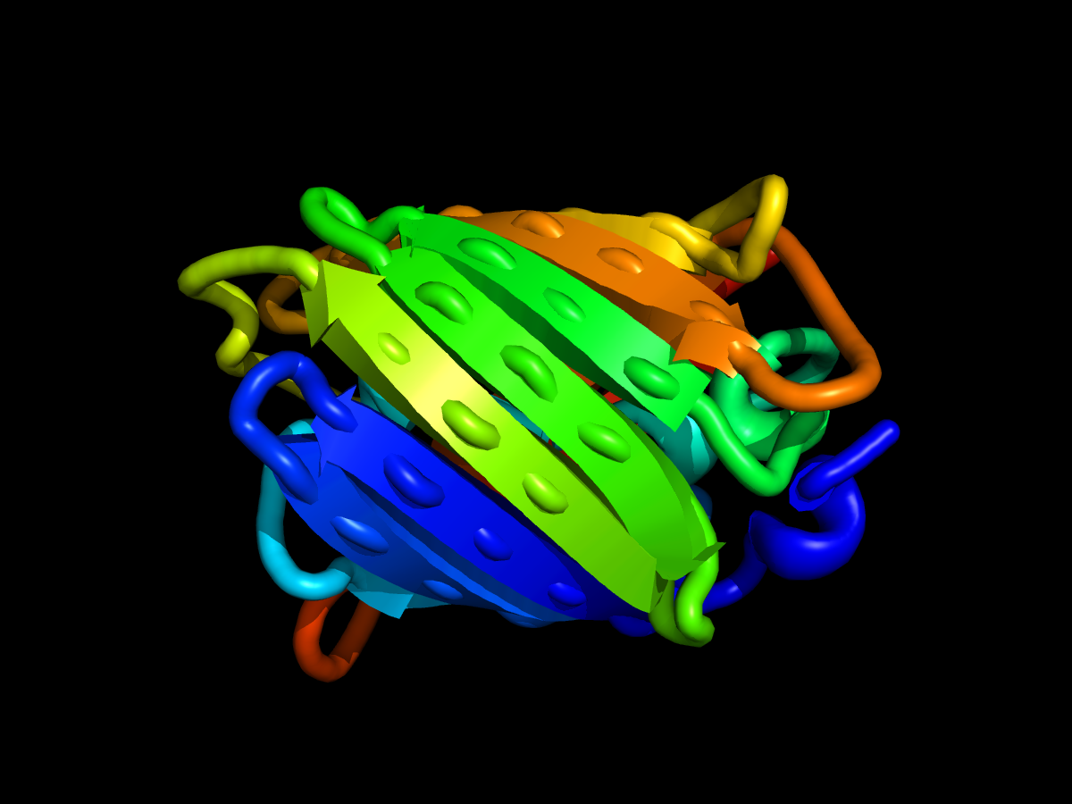
GFP's β-barrel with the chunky arrows applied. The bulges running along each strand are the spine tube passing through — the internal rebar, visible before it gets fused into one solid on export.
The name
My best friend in high school once shared an apartment with MC Chris, who voiced MC Pee Pants in Aqua Teen Hunger Force. I'm not saying that was the inspiration for the name of this project, but I'm not denying it either.
Provenance
Built on macOS using the open-source PyMOL available via Homebrew. Started with Antigravity, then Gemini Pro 3.1 until I ran out of tokens, then Claude Code (Sonnet 4.6 thinking). Tested with Claude Code and Gemini CLI. Conservation analysis uses the ColabFold public MMseqs2 API (please don't hammer it).
License
MIT.
1 maintainer

Download files
Download the file for your platform. If you're not sure which to choose, learn more about installing packages.
Source Distribution
Built Distribution
Filter files by name, interpreter, ABI, and platform.
If you're not sure about the file name format, learn more about wheel file names.
Copy a direct link to the current filters
File details
Details for the file mcpymol-1.5.1.tar.gz.
File metadata
- Download URL: mcpymol-1.5.1.tar.gz
- Upload date:
- Size: 6.9 MB
- Tags: Source
- Uploaded using Trusted Publishing? Yes
- Uploaded via:
twine/7.0.0 CPython/3.13.14
File hashes
| Algorithm | Hash digest | |
|---|---|---|
| SHA256 |
4f08777dbce86cf99e26ea4a989403716a0470f6037b791392f54d25c9d4f009
|
|
| MD5 |
36ff752ac10c1122993548a4f6044713
|
|
| BLAKE2b-256 |
b093a853dab2223e22807e5637808814b5b842fc8c23733259398a6b9f0c1127
|
Provenance
The following attestation bundles were made for mcpymol-1.5.1.tar.gz:
Publisher:
release.yml on chemrich/MCPymol
-
Statement:
-
Statement type:
https://in-toto.io/Statement/v1 -
Predicate type:
https://docs.pypi.org/attestations/publish/v1 -
Subject name:
mcpymol-1.5.1.tar.gz -
Subject digest:
4f08777dbce86cf99e26ea4a989403716a0470f6037b791392f54d25c9d4f009 - Sigstore transparency entry: 2387455228
- Sigstore integration time:
-
Permalink:
chemrich/MCPymol@2866da031b0eac3ee88c5b80ceec610c5778634c -
Branch / Tag:
refs/tags/v1.5.1 - Owner: https://github.com/chemrich
-
Access:
public
-
Token Issuer:
https://token.actions.githubusercontent.com -
Runner Environment:
github-hosted -
Publication workflow:
release.yml@2866da031b0eac3ee88c5b80ceec610c5778634c -
Trigger Event:
push
-
Statement type:
File details
Details for the file mcpymol-1.5.1-py3-none-any.whl.
File metadata
- Download URL: mcpymol-1.5.1-py3-none-any.whl
- Upload date:
- Size: 93.3 kB
- Tags: Python 3
- Uploaded using Trusted Publishing? Yes
- Uploaded via:
twine/7.0.0 CPython/3.13.14
File hashes
| Algorithm | Hash digest | |
|---|---|---|
| SHA256 |
e075e5884e47d74e8064941e8e8a501461cca95be0fe311cc2e4d6156215b495
|
|
| MD5 |
892466b0d791d757ae7d08ad8bc72c68
|
|
| BLAKE2b-256 |
c7e5a2e07182e9b3d791b1115c61894a981cc797f7ae8b41f8a9d12fa8d51117
|
Provenance
The following attestation bundles were made for mcpymol-1.5.1-py3-none-any.whl:
Publisher:
release.yml on chemrich/MCPymol
-
Statement:
-
Statement type:
https://in-toto.io/Statement/v1 -
Predicate type:
https://docs.pypi.org/attestations/publish/v1 -
Subject name:
mcpymol-1.5.1-py3-none-any.whl -
Subject digest:
e075e5884e47d74e8064941e8e8a501461cca95be0fe311cc2e4d6156215b495 - Sigstore transparency entry: 2387455230
- Sigstore integration time:
-
Permalink:
chemrich/MCPymol@2866da031b0eac3ee88c5b80ceec610c5778634c -
Branch / Tag:
refs/tags/v1.5.1 - Owner: https://github.com/chemrich
-
Access:
public
-
Token Issuer:
https://token.actions.githubusercontent.com -
Runner Environment:
github-hosted -
Publication workflow:
release.yml@2866da031b0eac3ee88c5b80ceec610c5778634c -
Trigger Event:
push
-
Statement type:














