
MCRand
MCRand is a library of Monte Carlo methods. Multidimensional integration, non-uniform random number generation, etc.
Random Number Generator
In the samples folder you can find a comparison between MCRand and Numpy for different probability distributions. Moreover, we use the program to generate random samples drawn from non-standard distributions. Anyway, we show here a quick guide to use MCRand library to generate the outputs of samples/pdf.py.
To use the MCRand library to generate random numbers we first need to import the random generator (RandGen). This step can be done in the following way
from mcrand import sample
Gaussian distribution
To generate gaussian distributed numbers with the MCRand random generator we first need to define the Gaussian PDF
def gaussian(x, mu, sigma):
	return (1/(np.sqrt(2*np.pi*sigma**2))) * np.exp(-(x-mu)**2/(2*sigma**2))
Then, MCRand can be used to generate N gaussian numbers from x0 to xf as follows
x0 = -5
xf = 5
N = 1000

sigma = 1
mu = 0

gaussian_sample = sample(gaussian, x0, xf, N, mu, sigma)
Finally to plot the histogram and the PDF we can use matplotlib.pyplot
import matplotlib.pyplot as plt

plt.hist(gaussian_sample, bins=30, density=True, color=(0,1,0,0.5), label='MCRand sample')
plt.plot(x, gaussian(x, mu, sigma), color='r', label=r'Gaussian PDF $\mu=%.2f$, $\sigma=%.2f$' % (mu,sigma))

Cauchy distribution
To generate a Cauchy distribution we need to define its PDF
def cauchy(x, x0, gamma):
	return 1 / (np.pi * gamma * (1 + ((x-x0)/(gamma))**2))
and then use the random number generator of MCRand as before
x0 = -10
xf = 10
N = 10**5

x0_cauchy = 0
gamma = 1

cauchy_sample = sample(gaussian, x0, xf, N, mu, sigma)
Finally we plot the histogram and the PDF
plt.hist(cauchy_sample, bins=50, density=True, color=(0,1,0,0.5), label='MCRand sample')
plt.plot(x, cauchy(x, x0_cauchy, gamma), color='r', label=r'Cauchy PDF $\gamma=%.2f$, $x_0=%.2f$' % (gamma, x0_cauchy))

From now on, we'll just write some code along with the output figures of the pdf.py file.
Exponential distribution
def exponential(x):
	return np.exp(-x)

x0 = 0
xf = 10
N = 10**5

rand = sample(exponential, x0, xf, N)

plt.hist(numpy_rand, bins=30, density=True, color=(0,0,1,0.8), label='NumPy sample')
plt.hist(rand, bins=30, density=True, color=(0,1,0,0.5), label='MCRand sample')

Rayleigh distribution
def rayleigh(x, sigma):
	return (x*np.exp(-(x**2)/(2*sigma**2))) / (sigma**2)

x0 = 0
xf = 4
sigma = 1
N = 10**5

rand = sample(rayleigh, x0, xf, N, sigma)

plt.hist(rand, bins=30, density=True, color=(0,1,0,0.5), label='MCRand sample')
plt.plot(x, rayleigh(x, sigma), color='r', label=r'Rayleigh PDF $\sigma=%.2f$' % sigma)

Maxwell-Boltzmann distribution
def maxwell_boltzmann(x, sigma):
	return (np.sqrt(2/np.pi))*(x**2*np.exp(-(x**2)/(2*sigma**2))) / (sigma**3)

x0 = 0
xf = 10
sigma = 2
N = 10**5

rand = sample(maxwell_boltzmann, x0, xf, N, sigma)

plt.hist(rand, bins=30, density=True, color=(0,1,0,0.5), label='MCRand sample')
plt.plot(x, maxwell_boltzmann(x, sigma), color='r', label=r'Maxwell-Boltzmann PDF $\sigma=%.2f$' % sigma)

Symmetric Maxwell-Boltzmann distribution
def symmetric_maxwell_boltzmann(x, sigma):
	return 0.5*(np.sqrt(2/np.pi))*(x**2*np.exp(-(x**2)/(2*sigma**2))) / (sigma**3)

x0 = -10
xf = 10
sigma = 2
N = 10**5

rand = sample(symmetric_maxwell_boltzmann, x0, xf, N, sigma)

plt.hist(rand, bins=40, density=True, color=(0,1,0,0.5), label='MCRand sample')
plt.plot(x, symmetric_maxwell_boltzmann(x, sigma), color='r', label=r'Maxwell-Boltzmann PDF $\sigma=%.2f$' % sigma)

Modified Rayleigh distribution
Finally we consider a invented probability distribution, given by the Rayleigh distribution multiplied by x. In some way we making a symmetric Rayleigh distribution. Then, this new distribution must be normalized, so the following equation must be acomplished:
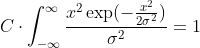
By nummeric integration it turns out that the normalization constant must be C=1/2.506628. Then we get the probability density function for this distribution.
Therefore, MCRand can be used to generate random numbers distributed following this distribution as follows
def invented(x, sigma):
	return (x**2*np.exp(-(x**2)/(2*sigma**2))) / (2.506628*sigma**2)

x0 = -4
xf = 4
sigma = 1
N = 10**5

rand = sample(invented, x0, xf, N, sigma)

plt.hist(rand, bins=40, density=True, color=(0,1,0,0.5), label='MCRand sample')
plt.plot(x, invented(x, sigma), color='r', label=r'Modified Rayleigh PDF $\sigma=%.2f$' % sigma)

Multidimensional Integration
To use the MCRand library to perform multidimensional integrals we first need to import the Integrate module. This step can be done in the following way
from mcrand import uniform_integration
Then, we must define the function to integrate in an NumPy ndarray supported way, so it must be defined generally. For instance let's imagine we want so solve the following integral:

Then we should define the function as
def func(x):
	return np.sum(np.power(x, 2))
so each element of the x array will represent a variable.
Finally, to get the result with its error we can run the following code
x0 = [0, 0]
xf = [2, 3]
N = 10**6

result = uniform_integration(func, x0, xf, N)

print(result)
The result is given in the following format
(25.99767534344232, 0.02023068196284685)
1 maintainer

Metadata
1 maintainer
Release files for mcrand 0.0.2
For a detailed explanation of source distributions (sdists) and built distributions (wheels), please see the package formats documentation.
Source distribution (sdist)
| File | Size | Uploaded | |
|---|---|---|---|
| mcrand-0.0.2.tar.gz | 5.2 kB | Details |
Built distribution (wheel)
| File | Interpreter | ABI | Platform | Reset |
|---|---|---|---|---|
| mcrand-0.0.2-py3-none-any.whl | Python 3 | none | any | Details |
Total release size: 22.9 kB
Release files / mcrand-0.0.2.tar.gz
| Download URL | mcrand-0.0.2.tar.gz |
|---|---|
| Size | 5.2 kB |
| Tags | Source |
|
SHA-256 checksum How to use checksums |
788a73d3cbe9b2c2a511c535e57e46e4a61f701b896ba5c8e8ff5d611a682669
|
|
BLAKE2b-256 checksum How to use checksums |
20468cb97adf0a87a9d501ad1735a63dcd14a8111f13528ab2312bc063029cab
|
| Upload date | |
|
Uploaded using Trusted Publishing? What is trusted publishing? |
No |
| Uploaded via |
twine/3.2.0 pkginfo/1.5.0.1 requests/2.23.0 setuptools/49.2.1 requests-toolbelt/0.9.1 tqdm/4.46.0 CPython/3.7.7
|
Release files / mcrand-0.0.2-py3-none-any.whl
| Download URL | mcrand-0.0.2-py3-none-any.whl |
|---|---|
| Size | 17.7 kB |
| Tags | Python 3 |
|
SHA-256 checksum How to use checksums |
3b52d5b040833308bbf7e558e21c151c60defc86d0279fa6be4eb2f5182e5d44
|
|
BLAKE2b-256 checksum How to use checksums |
025e5d32dcd2aa065d7ca3c34e10e5925b50f49baec4bffc7633345cd0e1864d
|
| Upload date | |
|
Uploaded using Trusted Publishing? What is trusted publishing? |
No |
| Uploaded via |
twine/3.2.0 pkginfo/1.5.0.1 requests/2.23.0 setuptools/49.2.1 requests-toolbelt/0.9.1 tqdm/4.46.0 CPython/3.7.7
|













