Visualization tool for (meta)genome assembly graphs

Project description
 MetagenomeScope


Interactive visualization tool for (meta)genome assembly graphs.
MetagenomeScope decomposes the graph into structural patterns and highlights these as annotations on the graph. By default it lays out the graph hierarchically, using Graphviz' dot algorithm.
MetagenomeScope also contains various functionalities for visualizing assembly graphs at larger scales -- for example, highlighting scaffold paths on the graph and drawing summary plots of the graph's structure.
This tool is still a work in progress, so please let us know if you have any feedback!
Screenshots
| Stool metagenome assembly (MetaCarvel) | Yeast genome assembly (Flye) |
|---|---|
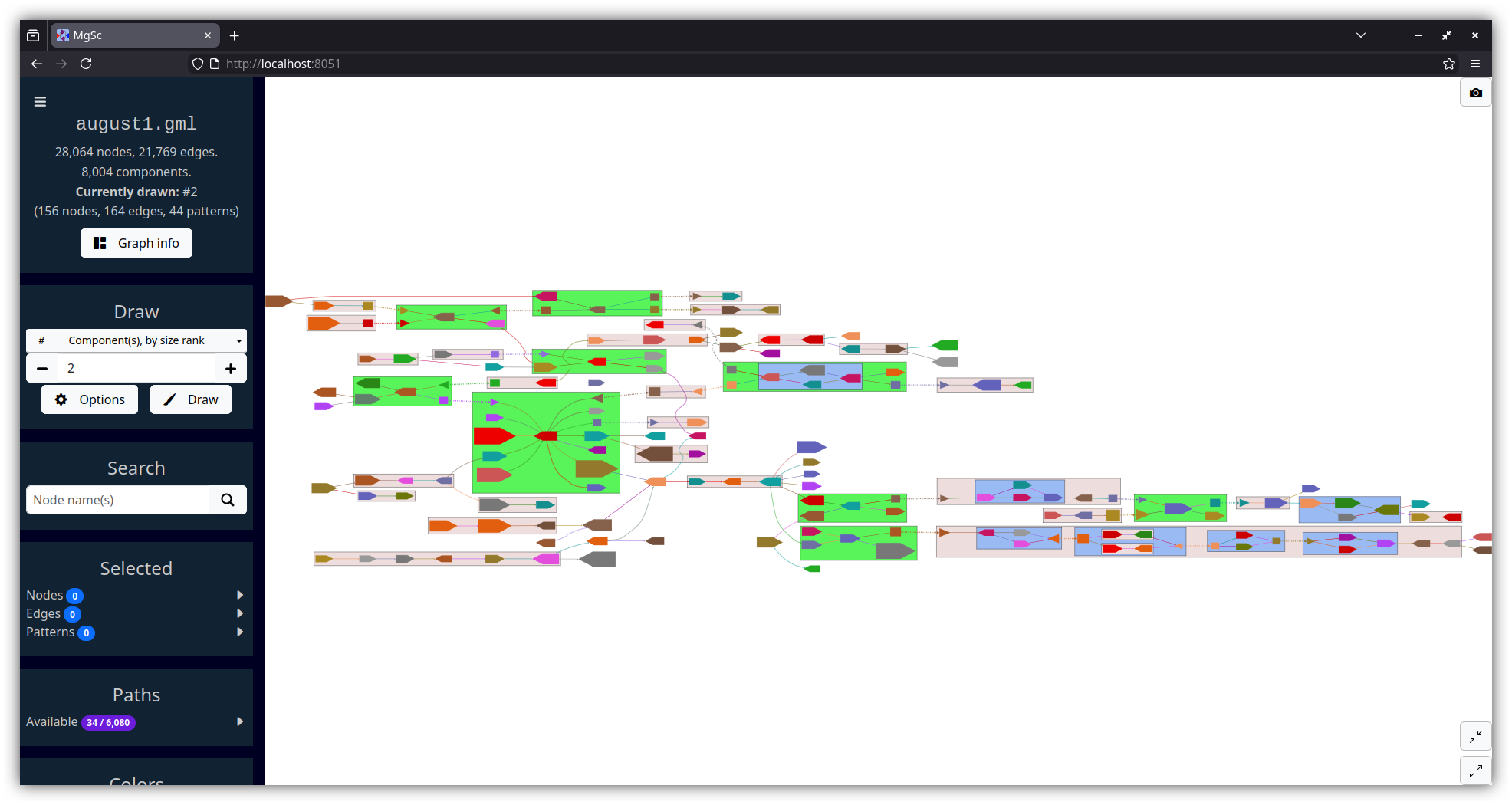 |
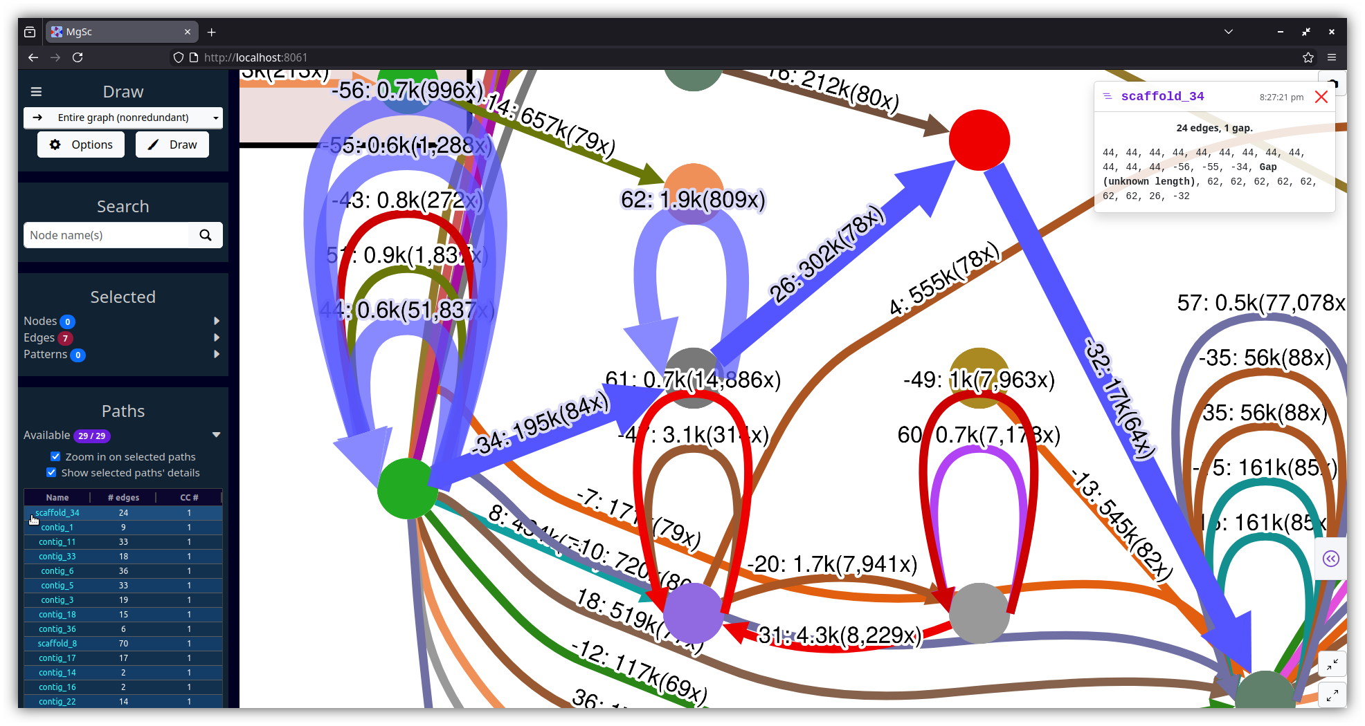 |
| Data source: SRS049959 | Data source: AGB |
| Summarizing graph structure in a treemap | Interactive charts of graph statistics |
|---|---|
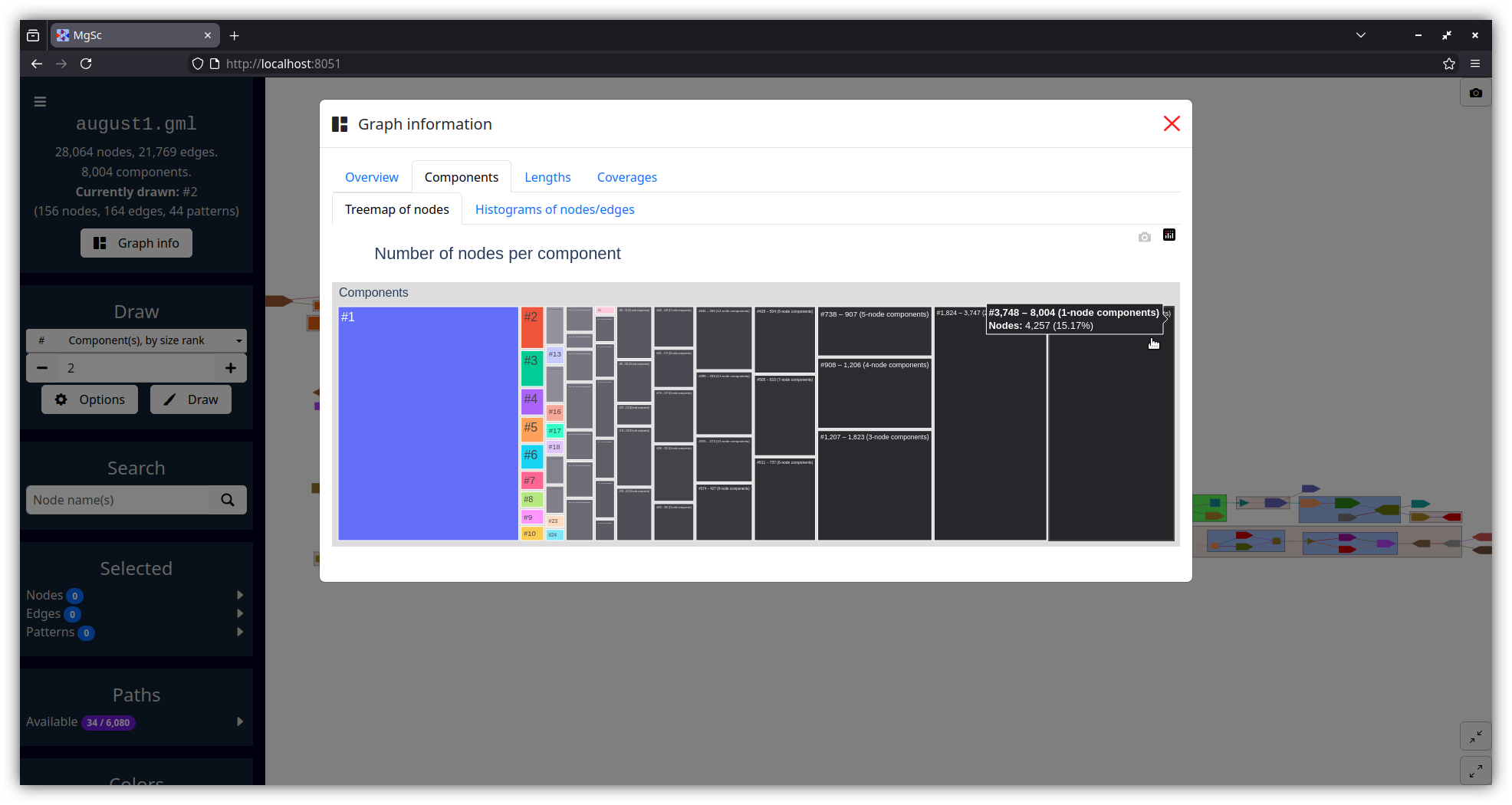 |
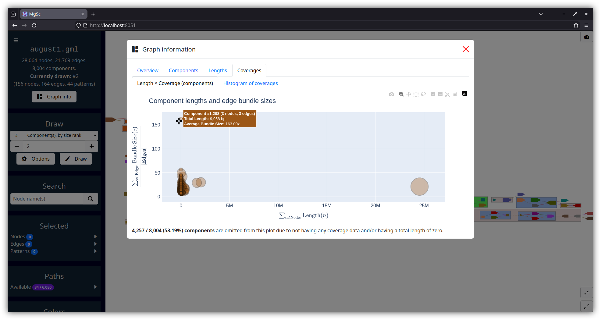 |
| Data source: SRS049959 | |
Installation
Using mamba:
mamba create -n mgsc -c conda-forge "python >= 3.8" pygraphviz
mamba activate mgsc
pip install metagenomescope
(We plan to put this on bioconda soon.)
Usage
Activate the mamba environment we just created and run:
mgsc -g graph.gfa
... where graph.gfa is a path to the assembly graph you want to visualize
(see information below on supported graph filetypes).
This will start a server using Dash.
The port number of the server defaults to 8050, so navigate
to localhost:8050 in a web browser to access the visualization.
All command-line options
Usage: mgsc [OPTIONS]

  Visualizes an assembly graph.

  Please visit https://github.com/marbl/MetagenomeScope for more information.

Options:
  -g, --graph FILE          In GFA, FASTG, DOT, GML, or LastGraph format.  [required]
  -a, --agp FILE            AGP file describing paths (e.g. scaffolds) in the graph.
  -i, --info FILE           Flye assembly_info.txt file describing contigs/scaffolds.
  -p, --port INTEGER RANGE  Server port number.  [default: 8050; 1024<=x<=65535]
  --verbose / --no-verbose  Log extra details.  [default: no-verbose]
  --debug / --no-debug      Use Dash's debug mode.  [default: no-debug]
  -v, --version             Show the version and exit.
  -h, --help                Show this message and exit.
Supported assembly graph filetypes
| Filetype | Generated by | Notes |
|---|---|---|
GFA (.gfa) |
Flye, LJA, hifiasm, verkko, ... | Both GFA 1 and GFA 2 files are accepted. Currently we visualize segments, links (GFA 1), non-containment edges (GFA 2), and paths of segments. |
FASTG (.fastg) |
SPAdes, MEGAHIT | Expects FASTG files produced by SPAdes or MEGAHIT. |
DOT (.dot, .gv) |
Flye, LJA | Expects DOT files produced by Flye or LJA. See "What filetype should I use for de Bruijn graphs?" in the FAQs below. |
GML (.gml) |
MetaCarvel | Expects GML files produced by MetaCarvel. |
LastGraph (.LastGraph) |
Velvet | Currently we just visualize the raw structure (nodes and arcs). |
Should you run into additional assembly graph filetypes you'd like us to support, feel free to open a GitHub issue.
Supported path filetypes
Paths can optionally be specified through any of the following inputs:
AGP files (-a)
See the AGP specification for details.
If your graph is in DOT format:
- We assume the
component_ids in column 6a of the AGP file correspond to edge IDs.
Otherwise:
- We assume the
component_ids correspond to node IDs.
Flye assembly_info.txt files (-i)
See Flye's documentation for details.
If your graph is in DOT format:
- We will visualize the edge-paths described in the
.txtfile.
If your graph is in GFA format:
-
The contigs in the GFA file should correspond to collapsed edge-paths in the
.txtfile, so we can't really visualize these edge-paths. -
However, we will extract contig information from the
.txtfile (e.g. coverage) and show it in the interface as node data.
P-lines in GFA 1 files, or O-lines in GFA 2 files (-g)
See the GFA 1 and GFA 2 specifications for details.
Currently, we only show segments on GFA paths (not edges, gaps, etc.)
Example datasets
Flye (DOT file, 61 nodes, 122 edges): S. cerevisiae (yeast)
This data is from AGB's GitHub repository.
wget https://raw.githubusercontent.com/marbl/MetagenomeScope/refs/heads/main/metagenomescope/tests/input/flye_yeast.gv
wget https://raw.githubusercontent.com/marbl/MetagenomeScope/refs/heads/main/metagenomescope/tests/input/flye_yeast_assembly_info.txt
mgsc -g flye_yeast.gv -i flye_yeast_assembly_info.txt
Velvet (LastGraph file, 558 nodes, 664 edges): E. coli
This is an example graph from Bandage. Note that the original sequences have been removed to save space.
wget https://raw.githubusercontent.com/marbl/MetagenomeScope/refs/heads/main/metagenomescope/tests/input/E_coli_LastGraph
mgsc -g E_coli_LastGraph
Hodgepodge of other test datasets
See the metagenomescope/tests/input/
directory.
FAQs
Reverse-complementary sequences
FAQ 1. How do you handle reverse-complementary nodes/edges?
The answer to this depends on the filetype of the graph you are using.
"Explicit" graph filetypes (FASTG, DOT, GML)
When MetagenomeScope reads in FASTG, DOT, and GML files, it assumes that these files explicitly describe all of the nodes and edges in the graph. So, let's say you give MetagenomeScope the following DOT file:
digraph g {
  1 -> 2 [label="edge1 A99(2.4)"];
}
We will interpret this as a graph with two nodes (1, 2) and one edge
(1 -> 2).
"Implicit" graph filetypes (GFA, LastGraph)
However, for GFA and LastGraph files, MetagenomeScope cannot make the assumption that these files explicitly describe all of the nodes and edges in the graph. In these files, each declaration of a node / edge (in GFA parlance, "segment" / "link"; in LastGraph parlance, "node" / "arc") also declares this node / edge's reverse complement.
So, let's say you give MetagenomeScope the following GFA file (based on this example):
H	VN:Z:1.0
S	1	CGATGCAA
S	2	TGCAAAGTAC
L	1	+	2	+	5M
We will interpret this as a graph with four nodes (1, -1, 2, -2)
and two edges (1 -> 2, -2 -> -1). The presence of node X
"implies"
the existence of the reverse complement node -X, and the presence of edge
X -> Y "implies" the existence of the reverse complement edge -Y -> -X.
Interpreting the graph file in this way is analogous to
how "double mode" works in Bandage.
Based on the FASTG specification, shouldn't FASTG be an "implicit" instead of an "explicit" filetype?
It's complicated. The way I interpret the FASTG specification, each declaration of an edge sequence implicitly also declares this edge sequence's reverse complement; however, this is not the case for "adjacencies" between edge sequences.
In any case, the "dialect" of FASTG files produced by SPAdes and MEGAHIT lists edge sequences and their reverse complements (as well as adjacencies between edge sequences and their reverse complements) separately. Because of this, we consider FASTG to be an "explicit" filetype. (See pyfastg's documentation for details on how we handle reverse complements in FASTG files.)
FAQ 2. Why does my graph have node X and -X in the same component?
One common reason this happens is the presence of palindromic sequences: these can cause both a sequence and its reverse-complement to be connected to each other.
This often occurs with the big ("hairball") component in an assembly graph.
FAQ 3. What happens if an edge is its own reverse complement?
(This assumes that you have read FAQ 1.)
This can happen if an edge exists from X -> -X or from -X -> X in an
"implicit" graph file (GFA / LastGraph). Consider
this GFA file:
H	VN:Z:1.0
S	1	AAA
S	2	ACG
S	3	CAT
S	4	TTT
L	1	+	1	+	2M
L	2	+	2	-	2M
L	3	-	3	+	2M
L	4	-	4	-	2M
Since this GFA file contains four "link" lines, we might think at first that the corresponding graph
contains 4 × 2 = 8 edges. However, the graph only contains 6 unique
edges. This is because the reverse complement of 2 -> -2 is itself:
we know from above that X -> Y implies -Y -> -X, but
-(-2) -> -(2) is equal to 2 -> -2! The same goes for -3 -> 3:
-(3) -> -(-3) is equal to -3 -> 3.
Both of these edges "imply" themselves as their own reverse complements!
How do we handle this situation? As of writing, when MetagenomeScope visualizes these graphs it will only draw one copy of these "self-implying" edges. This matches the original visualization of this graph, and also matches Bandage's visualization of this GFA file.
Notably, since we assume that "explicit" graph files (FASTG / DOT / GML)
explicitly define all of the nodes and edges in their graph, MetagenomeScope doesn't do anything
special for this case for these files. (If your DOT file describes one edge
from X -> -X, then that's fine; if it describes two or more edges from X -> -X,
then that's also fine, and we'll visualize all of them.)
Graph structure
FAQ 4. What do you mean by a component's "size rank"?
Given a graph with N connected components: we sort these components by the number of nodes they contain, from high to low. We then assign each of these components a size rank, a number from 1 to N: the component with size rank #1 corresponds to the largest component, and the component with size rank #N corresponds to the smallest component.
Often, we only care about looking at individual components in a graph -- laying out and drawing the entire graph is not always a good idea when the graph is massive. Component size ranks are a nice way of formalizing this.
Some details about component size ranks, if you are interested:
-
The numbers shown in the treemap (accessible in the "Graph info" dialog) correspond exactly to component size ranks. So, the rectangle labelled #1 in the treemap corresponds to the largest component, the rectangle labelled #2 corresponds to the second-largest component, etc.
-
The exact component sorting functionality accounts for ties by using four different sorting criteria, in the following order. Ties at one level cause later levels to be considered for breaking ties.
- the number of "full" nodes in the component (treating a pair of split nodes 40-L → 40-R as a single node)
- the number of "total" nodes in the component (treating a pair of split nodes 40-L → 40-R as two nodes)
- the number of "total" edges in the component (including both real edges and "fake" edges between pairs of split nodes like 40-L → 40-R)
- the number of patterns in the component
FAQ 5. Can my graphs have parallel edges?
Yes! MetagenomeScope supports
multigraphs. If your assembly graph
file describes more than one edge from X -> Y, then MetagenomeScope will
visualize all of these "parallel" edges. (This is mostly useful when visualizing
de Bruijn graphs.)
Notably, parallel edges not supported right now for FASTG files. I don't think I've ever seen any FASTG files that have parallel edges, so I don't think this is a big priority, but please let me know if you would like us to add support for it.
FAQ 6. What filetype should I use for de Bruijn graphs?
If you are visualizing output from LJA or Flye, you may want to use a DOT file instead of a GFA / FASTG file as input.
This is because GFA and FASTG are not ideal for representing graphs in which sequences are stored on edges rather than nodes (i.e. de Bruijn / repeat graphs). The DOT files output by Flye and LJA should contain the original structure of these graphs (in which edges and nodes in the visualization actually correspond to edges and nodes in the original graph, respectively); the GFA / FASTG files usually represent altered versions in which nodes and edges have been swapped, which is not always an ideal representation (especially if you are doing something where you really care about the structure of the original graph).
That being said, please note that -- if you are using an assembler that outputs graphs in different filetypes -- these files may have additional differences beyond the usual filetype differences. For example, Flye's GFA and DOT files can have slightly different coverages, since Flye produces them at different times in its pipeline.
Filetypes
FAQ 7. I got an error saying Custom record types are not supported in GFA1?
Some assemblers include additional kinds of lines in their output GFA files. For example,
hifiasm and hifiasm-meta include A-lines describing alignments.
These "custom" lines can cause problems when parsing these graphs, because they may not be technically allowed in certain GFA versions.
The simplest way around this is just deleting or commenting out these custom lines. Here is an examle of commenting out the A-lines in hifiasm GFA files using sed:
sed -i -e 's/^A/#A/' hifiasm-out.p_ctg.gfa
Eventually I'd like to implement a better solution for this...
Patterns
FAQ 8. How can I run the pattern decomposition process programmatically?
Creating a metagenomescope.graph.AssemblyGraph object will automatically run the decomposition process:
>>> from metagenomescope.graph import AssemblyGraph
>>> ag = AssemblyGraph("graph.gfa")  # replace with your graph's filepath
At this point:
-
The "decomposed graph" (where patterns are collapsed into nodes) is represented by
ag.decomposed_graph(a NetworkXMultiDiGraph). -
The "original graph" (i.e. with all patterns fully uncollapsed, revealing all "original" nodes and edges) is represented by
ag.graph(also a NetworkXMultiDiGraph)- Note that this graph will still include split nodes and fake edges, if any remain after the decomposition process.
-
All nodes, edges, and patterns will have unique integer IDs. These IDs can be used to look up information about nodes, edges, and patterns in the
ag.nodeid2obj,ag.edgeid2obj, andag.pattid2objdictionaries, respectively.
Some examples of analyzing the decomposition results:
>>> from metagenomescope.graph import AssemblyGraph
>>> ag = AssemblyGraph("metagenomescope/tests/input/E_coli_LastGraph")
>>> # Inspect nodes, edges, and patterns
>>> ag.nodeid2obj
{0: Node 0 (name: 1),
 1: Node 1 (name: -1),
 2: Node 2 (name: 2),
 ...}
>>> ag.edgeid2obj
{558: Edge 558 (orig: 0 -> 244; new: 0 -> 244; dec: 0 -> 1421),
 559: Edge 559 (orig: 1 -> 342; new: 1 -> 342; dec: 1527 -> 342),
 560: Edge 560 (orig: 2 -> 477; new: 2 -> 477; dec: 2 -> 477),
 ...}
>>> ag.pattid2obj
{1222: bubble1222 containing nodes [33, 283, 395, 39] from [33] to [39],
 1227: bubble1227 containing nodes [34, 76, 382, 303] from [34] to [76],
 1232: bubble1232 containing nodes [40, 43, 35, 501] from [35] to [43],
 ...}
>>> # Go through just the bubble patterns
>>> ag.bubbles
[bubble1222 containing nodes [33, 283, 395, 39] from [33] to [39],
 bubble1227 containing nodes [34, 76, 382, 303] from [34] to [76],
 bubble1232 containing nodes [40, 43, 35, 501] from [35] to [43],
 ...]
>>> # Look up a node by name (if a node was split, this will list both halves)
>>> ag.nodename2objs
defaultdict(<class 'list'>,
            {'1': [Node 0 (name: 1)],
             '-1': [Node 1 (name: -1)],
             '2': [Node 2 (name: 2)],
             ...
             '40-R': [Node 78 (name: 40-R)],
             '40': [Node 78 (name: 40-R), Node 1259 (name: 40-L)],
             '40-L': [Node 1259 (name: 40-L)],
             ...})
>>> # Examine split nodes
>>> for n in ag.nodeid2obj.values():
...     if n.split is not None:
...         print(n)
Node 32 (name: 17-L)
Node 33 (name: -17-R)
Node 34 (name: 18-R)
...
>>> # Distinguish fake from real edges
>>> for e in ag.edgeid2obj.values():
...     print(e, e.is_fake)
Edge 558 (orig: 0 -> 244; new: 0 -> 244; dec: 0 -> 1421) False
Edge 559 (orig: 1 -> 342; new: 1 -> 342; dec: 1527 -> 342) False
...
Edge*1634 (orig: 348 -> 1633; new: 348 -> 1633; dec: 1628 -> 1666) True
Edge*1639 (orig: 1638 -> 451; new: 1638 -> 451; dec: 1671 -> 1635) True
This interface should remain relatively stable, although I may change things slightly as development continues. If you have any questions, please reach out.
Performance
FAQ 9. What's the biggest possible graph I can visualize?
We're still figuring that out. There are two main bottlenecks I am aware of:
-
Laying out the graph.
-
We usually only lay out one component at a time, so generally the problem comes with laying out the large "hairball" component(s) of the graph, if any.
-
When you get to the order of, say, thousands of nodes, laying out a component will probably become somewhat slow (especially if you select the
Lay out patterns recursivelyoption in the draw options dialog). -
To my understanding, a big factor here is the ratio of nodes to edges: when there are many more edges than nodes in a component (indicating a very densely connected structure), Graphviz has to do a lot of work to position things properly.
-
-
Drawing the graph's elements.
-
Cytoscape.js has a lot of optimizations built-in, but I think there are some inherent limitations of drawing using a HTML canvas.
-
With graphs containing thousands of nodes, interaction (e.g. zooming, panning) starts to feel a bit sluggish.
-
I have some ideas for dealing with these bottlenecks, but thankfully there are already ways around both of these issues. Some approaches that may be helpful:
-
Assuming that your graph has multiple components, check out the
Componentstab in theGraph infodialog to see how big these components are. If component #1 (the largest one) contains more than, say, 10,000 nodes, you may want to start off with analyzing the smaller components. -
You don't need to draw entire components at once. Try using the
Around certain node(s)drawing method (in the dropdown inside theDrawsection): if you are interested in just certain neighborhood(s) in a massive component, you can enter in a list of nodes here (and some distance around them) and we'll just draw the corresponding neighborhoods. (Inspired by Bandage :) -
Turning off labels might be helpful?
-
Although probably not by that much, since we already use Cytoscape.js' functionality to hide labels when you're zoomed out from the graph.
-
So... if you set a really big label font size and zoom the graph out really far, then labels could cause performance issues.
-
Known issues
-
Edge flattening: Cytoscape.js (the library we use to visualize graphs in the browser) can sometimes determine that the control points used to draw certain complex edges are invalid. This can happen as you adjust the visualization after drawing (e.g. by selecting nodes or moving them around).
To prevent these "invalid" edges from being hidden, MetagenomeScope will detect them and "flatten" them into simple Bezier edges (usually straight lines). This way, we can at least draw something for each edge in the graph.
-
Long graphs: Graph layouts that form a long horizontal or vertical line may break Cytoscape.js' rendering process (#262). If this happens to you, you can refresh the page to get Cytoscape.js working again.
Development documentation
See CONTRIBUTING.md.
License
MetagenomeScope is licensed under the GNU GPL, version 3.
MetagenomeScope's code is distributed with Bootstrap and Bootstrap Icons. Please see the metagenomescope/assets/vendor/licenses/ directory for copies of these tools' licenses.
Acknowledgements
Thanks to various people in the Pop, Knight, and Pevzner Labs over the years for their kind feedback and helpful suggestions.
Thanks also to the developers of the many excellent open-source software packages used by MetagenomeScope. In particular, Graphviz (graph layout), Cytoscape.js (interactive graph drawing), and Dash (application framework) have been extremely helpful tools throughout the development of this project.
Contact
Please open a GitHub issue if you have any questions or suggestions.
Release history Release notifications | RSS feed


Download files
Download the file for your platform. If you're not sure which to choose, learn more about installing packages.
Source Distribution
Built Distribution
Filter files by name, interpreter, ABI, and platform.
If you're not sure about the file name format, learn more about wheel file names.
Copy a direct link to the current filters
File details
Details for the file metagenomescope-1.0.0.tar.gz.
File metadata
- Download URL: metagenomescope-1.0.0.tar.gz
- Upload date:
- Size: 698.7 kB
- Tags: Source
- Uploaded using Trusted Publishing? No
- Uploaded via: Hatch/1.16.3 cpython/3.13.9 HTTPX/0.28.1
File hashes
| Algorithm | Hash digest | |
|---|---|---|
| SHA256 |
ccf76034faf315c8a1b3e56b940903170eca068f9e03ab8391857146f29aea88
|
|
| MD5 |
6c3affabff7282e623e05a5123f28da7
|
|
| BLAKE2b-256 |
b19ea58b6c9bed45fd744ac4bf420627111edafe20b5ed08bbc104329306b2fb
|
File details
Details for the file metagenomescope-1.0.0-py3-none-any.whl.
File metadata
- Download URL: metagenomescope-1.0.0-py3-none-any.whl
- Upload date:
- Size: 626.2 kB
- Tags: Python 3
- Uploaded using Trusted Publishing? No
- Uploaded via: Hatch/1.16.3 cpython/3.13.9 HTTPX/0.28.1
File hashes
| Algorithm | Hash digest | |
|---|---|---|
| SHA256 |
40785a499038a41eee4d840cb15b520a960a02db946f4ec77292188e72ea9ea0
|
|
| MD5 |
44f8ae57a30288d9e6a204737063242b
|
|
| BLAKE2b-256 |
7236f951f9f2376d70044bfe64f72862ba963d5c5f308ef601fa144d64605dfb
|


