

metalog-jax
GPU-accelerated metalog distributions for modern probabilistic modeling


Installation • Quick Start • Features • Documentation • Citation
metalog-jax
The Problem
Traditional probability distributions often fail to model real-world data accurately. You find yourself:
- Trying multiple distributions, hoping one fits
- Truncating distributions to enforce bounds
- Using mixture models that are hard to interpret
- Writing custom likelihood functions for edge cases
What if one distribution family could fit virtually any continuous data?
The Solution
metalog-jax implements the Metalog distribution - a revolutionary approach to probability modeling introduced by Tom Keelin (2016). Metalogs are a continuous, semi-parametric family that can represent virtually any probability distribution through quantile-based fitting.
import jax.numpy as jnp
from metalog_jax.base import MetalogInputData, MetalogParameters
from metalog_jax.base import MetalogBoundedness, MetalogFitMethod
from metalog_jax.metalog import fit
from metalog_jax.utils import DEFAULT_Y

# Your data
data = jnp.array([2.1, 3.5, 4.2, 5.8, 6.1, 7.3, 8.9, 12.4, 15.2, 18.7])

# Create validated input data
input_data = MetalogInputData.from_values(data, DEFAULT_Y, precomputed_quantiles=False)

# Configure metalog parameters (Feasible always returns a valid distribution)
params = MetalogParameters(
    boundedness=MetalogBoundedness.STRICTLY_LOWER_BOUND,
    lower_bound=0.0,
    upper_bound=0.0,
    method=MetalogFitMethod.Feasible,
    num_terms=5,
)

# Fit the metalog distribution
metalog = fit(input_data, params)

# Use it like any scipy distribution
median = metalog.ppf(jnp.array([0.5]))   # Quantile function
density = metalog.pdf(jnp.array([0.5]))  # Probability density
cumulative = metalog.cdf(10.0)           # CDF at x=10
Why metalog-jax?
| Feature | metalog-jax | pymetalog |
|---|---|---|
| GPU acceleration | Yes | No |
| Automatic differentiation | Yes | No |
| JIT compilation | Yes | No |
| Bounded distribution support | Yes | Yes |
| Multiple fit methods | Yes (OLS, LASSO, Feasible) | OLS only |
| Always-feasible fitting (Baucells et al. 2025) | Yes | No |
| Hyperparameter grid search | Yes (vectorized) | No |
| Serialization (save/load) | Yes | No |
| Active development | Yes | No |
Installation
Using pip
pip install metalog-jax
Using uv (recommended)
uv add metalog-jax
With GPU support (CUDA 12)
# pip
pip install "metalog-jax[gpu]"

# uv
uv add "metalog-jax[gpu]"
Note: GPU support requires Linux (or WSL2 on Windows) with CUDA 12. JAX does not publish CUDA wheels for native Windows.
From source
git clone https://github.com/tjefferies/metalog_jax.git
cd metalog_jax
make install    # Install all dependencies
Requirements
- Python >= 3.11
- JAX >= 0.8.0
- Flax >= 0.12.0
- Chex >= 0.1.91
- Plotly >= 6.4.0
Quick Start
Fitting a Distribution
import jax.numpy as jnp
from metalog_jax.base import MetalogInputData, MetalogParameters
from metalog_jax.base import MetalogBoundedness, MetalogFitMethod
from metalog_jax.metalog import fit
from metalog_jax.utils import DEFAULT_Y

# Sample data (e.g., response times in microseconds)
response_times = jnp.array([
    45, 52, 58, 61, 67, 72, 78, 85, 93, 102,
    115, 128, 145, 167, 195, 238, 312, 456, 623, 892
])

# Create validated input data
data = MetalogInputData.from_values(response_times, DEFAULT_Y, precomputed_quantiles=False)

# Configure the metalog (bounded below by 0)
params = MetalogParameters(
    boundedness=MetalogBoundedness.STRICTLY_LOWER_BOUND,
    lower_bound=0.0,
    upper_bound=0.0,
    method=MetalogFitMethod.Feasible,
    num_terms=5,
)

# Fit the distribution
metalog = fit(data, params)

# Analyze your distribution
print(f"Median response time: {float(metalog.ppf(jnp.array([0.5]))[0]):.1f} ms")
print(f"95th percentile: {float(metalog.ppf(jnp.array([0.95]))[0]):.1f} ms")
print(f"99th percentile: {float(metalog.ppf(jnp.array([0.99]))[0]):.1f} ms")
Working with Bounded Data
Metalog natively supports four boundedness types:
from metalog_jax.base import MetalogParameters, MetalogBoundedness, MetalogFitMethod

# Unbounded: support on (-inf, +inf)
# Example: temperature anomalies, returns
params = MetalogParameters(
    boundedness=MetalogBoundedness.UNBOUNDED,
    lower_bound=0.0,  # ignored
    upper_bound=0.0,  # ignored
    method=MetalogFitMethod.Feasible,
    num_terms=5,
)

# Lower-bounded: support on (lower_bound, +inf)
# Example: response times, prices, distances
params = MetalogParameters(
    boundedness=MetalogBoundedness.STRICTLY_LOWER_BOUND,
    lower_bound=0.0,
    upper_bound=0.0,  # ignored
    method=MetalogFitMethod.Feasible,
    num_terms=5,
)

# Upper-bounded: support on (-inf, upper_bound)
# Example: time until deadline, remaining capacity
params = MetalogParameters(
    boundedness=MetalogBoundedness.STRICTLY_UPPER_BOUND,
    lower_bound=0.0,  # ignored
    upper_bound=100.0,
    method=MetalogFitMethod.Feasible,
    num_terms=5,
)

# Fully bounded: support on (lower_bound, upper_bound)
# Example: percentages, probabilities, test scores
params = MetalogParameters(
    boundedness=MetalogBoundedness.BOUNDED,
    lower_bound=0.0,
    upper_bound=100.0,
    method=MetalogFitMethod.Feasible,
    num_terms=5,
)
Choosing a Fit Method
Start with MetalogFitMethod.Feasible. Set MetalogParameters.method to one of:
| Method | Use when | Hyperparameters |
|---|---|---|
MetalogFitMethod.Feasible |
Recommended default. Always returns a valid distribution: the OLS fit when it is valid, otherwise the closest valid metalog | None |
MetalogFitMethod.OLS |
You need fit_grid, which supports only OLS and LASSO. Closed-form least squares; fit raises if the density is negative on its check grid |
None |
MetalogFitMethod.Lasso |
Noisy data or many terms; L1 regularization shrinks unneeded coefficients | LassoParameters |
Always-Feasible Fitting
MetalogFitMethod.Feasible is the recommended fit method. It returns the best
least-squares fit among valid metalogs: the coefficient vector a* from Baucells,
Chrisman, Keelin and Xu (2025),
"On the Properties of the Metalog Distribution",
solved as a semi-infinite QP by the exchange method. It works with every boundedness option.
metalog-jax keeps the term assignment of Keelin (2016). The paper's Metalog 2.0
assignment differs from the 7th term on: for 7, 11, 15, ... terms the two span
different functions, and for other term counts the same functions with the
coefficients in a different order. The feasibility algorithms apply to both, and
best_feasible_fit(x, y, k, order=TermOrder.METALOG_2) fits the paper's
parameterization. For bounded and semi-bounded metalogs the fit, like OLS, is least
squares on the log- or logit-transformed quantiles (the paper's Section 4.10); the
back-transform keeps it valid.
Plain least squares (OLS) can return coefficients whose "density" goes negative
somewhere, which is more likely as you add terms. fit checks OLS results on a grid of
probabilities and raises. Feasible never returns an invalid distribution: every result
is certified by the exact check below, and fit raises if certification fails.
params = MetalogParameters(
    boundedness=MetalogBoundedness.UNBOUNDED,
    method=MetalogFitMethod.Feasible,
    lower_bound=0.0,
    upper_bound=0.0,
    num_terms=4,
)
metalog = fit(input_data, params)  # density is non-negative everywhere
metalog_jax.feasibility also exposes the underlying tools, all jit/vmap compatible:
from metalog_jax.feasibility import best_feasible_fit, check_feasibility, get_engine, summary_stats

res = best_feasible_fit(x, y, num_terms=6)            # a*, RSS, iterations, certificate
report = check_feasibility(get_engine(6), res.a_star)  # exact test: roots of M'', modes, tails
stats = summary_stats(get_engine(6), res.a_star)       # exact mean/variance/skewness/kurtosis
check_feasibility is exact rather than grid-based (Algorithm 1 of the paper), so it
cannot miss a negative-density region, including ones within 1e-7 of either tail. Every
sign it tests is decided exactly up to floating-point rounding, whatever the scale of the
coefficients.
When the OLS fit is already valid, Feasible returns exactly the OLS coefficients, so
choosing it costs nothing in fit quality; it only departs from OLS when OLS is invalid.
It takes no regression_hyperparams (passing them raises a TypeError).
Fitting Many Datasets with Feasible
fit_grid raises a ValueError for Feasible, because it varies the number of terms
inside vmap and the feasible solver needs it fixed at compile time. Use
fit_grid_datasets instead: it fits a whole batch in one call, and you loop over term
counts in Python.
import jax.numpy as jnp
from metalog_jax.grid_search import extract_metalog, fit_grid_datasets

# batched_x, batched_y: shape (n_datasets, n_quantiles)
params = MetalogParameters(
    boundedness=MetalogBoundedness.STRICTLY_LOWER_BOUND,
    lower_bound=0.0,
    upper_bound=0.0,
    method=MetalogFitMethod.Feasible,
    num_terms=10,
)

# Fixed number of terms: one vmapped call over all datasets
result = fit_grid_datasets(batched_x, batched_y, params)  # a: (n_datasets, 10)

# Different numbers of terms: one call per term count (each compiles once)
num_terms_list = [4, 6, 8, 10, 12]
results = {
    k: fit_grid_datasets(batched_x, batched_y, params.replace(num_terms=k))
    for k in num_terms_list
}
ks = jnp.stack([results[k].ks_dist for k in num_terms_list], axis=1)  # (n_datasets, n_terms)

# Best term count per dataset, as ready-to-use Metalog objects
best = jnp.argmin(ks, axis=1)
metalogs = [extract_metalog(results[num_terms_list[int(j)]], i) for i, j in enumerate(best)]
See examples/feasible_fits.py for a full walkthrough that
also audits the OLS fits with check_feasibility. On its five test datasets, 3 of the
10-term OLS fits are invalid distributions; Feasible fixes all of them.
Scaling to Many Datasets
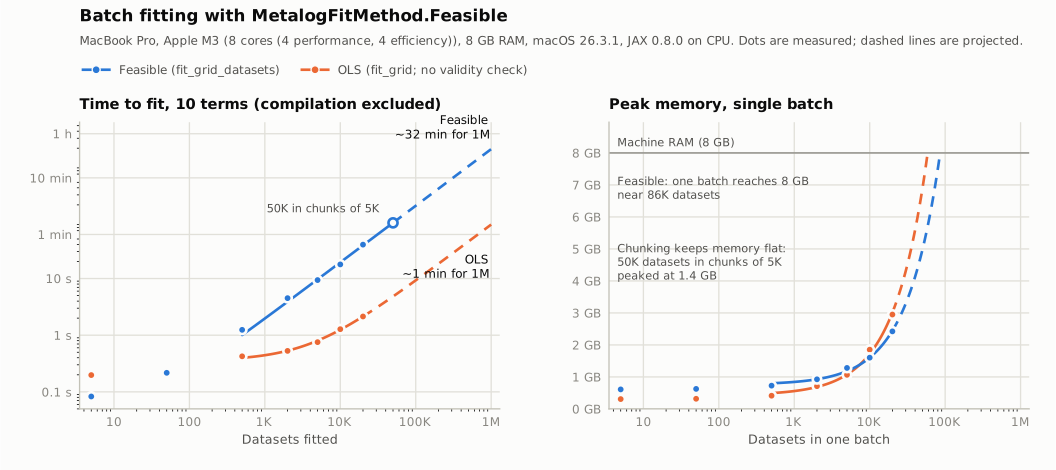
Measured with fit_grid_datasets on a MacBook Pro (Apple M3, 8 cores: 4 performance
and 4 efficiency, 8 GB unified memory), macOS 26.3.1, Python 3.13.7, JAX 0.8.0 on the
CPU backend (no GPU). Each dataset is 200 samples from one of the five distribution
families in examples/feasible_fits.py, summarized at the
105 DEFAULT_Y quantiles and fitted with a lower bound of 0. Times exclude the one-time
compilation, which takes 2-6 s per term count and batch shape.
| Datasets (10 terms) | Time | Per dataset | Peak memory |
|---|---|---|---|
| 5 | 0.08 s | 16.6 ms | 0.61 GB |
| 50 | 0.22 s | 4.3 ms | 0.62 GB |
| 500 | 1.24 s | 2.5 ms | 0.73 GB |
| 2,000 | 4.51 s | 2.3 ms | 0.92 GB |
| 5,000 | 9.41 s | 1.9 ms | 1.28 GB |
| 10,000 | 17.8 s | 1.8 ms | 1.60 GB |
| 20,000 | 39.7 s | 2.0 ms | 2.42 GB |
| 50,000 (10 chunks of 5,000) | 96.3 s | 1.9 ms | 1.43 GB |
The number of terms matters more than the number of datasets. At 5,000 datasets the time per dataset is:
| Terms | 4 | 6 | 8 | 10 | 12 |
|---|---|---|---|---|---|
| Per dataset | 0.19 ms | 0.69 ms | 1.22 ms | 1.88 ms | 3.10 ms |
Extrapolating (dashed lines in the chart; linear fits to batches of 500 or more):
- Throughput: about 1.9 ms per dataset at 10 terms, or roughly 1.9 million datasets per hour on this laptop; one million datasets take about 32 minutes. Comparing all five term counts, as in the example's second case, costs about 7 ms per dataset (about 2 hours per million).
- Memory: one batch needs about 0.76 GB plus 88 KB per dataset, so it would reach this machine's 8 GB near 86,000 datasets. Split larger jobs into fixed-size chunks instead: 5,000-10,000 datasets per chunk was the fastest per dataset here, memory stays flat (50,000 datasets in chunks of 5,000 peaked at 1.4 GB), and every chunk reuses one compiled shape. Pad the last chunk to the same size to avoid a recompile.
- OLS for comparison:
fit_gridwith OLS is about 20 times faster (0.09 ms per dataset) but does not check validity. At 10 terms, 65% of these datasets' OLS fits are invalid distributions, andfit_grid_datasetswith OLS raises for the whole batch if any one fit is invalid.
GPU performance was not measured. To reproduce, or to rerun on your own hardware:
uv run python benchmarks/feasible_scaling/bench.py feasible 5000 10 3       # one batch
uv run python benchmarks/feasible_scaling/bench_chunked.py 50000 5000 10    # chunked
uv run --with matplotlib python benchmarks/feasible_scaling/plot.py \
    benchmarks/feasible_scaling/results.json docs/source/_static           # redraw the chart
Regularized Fitting
For noisy data or when using many terms, LASSO regularization improves stability:
from metalog_jax.base import MetalogInputData, MetalogParameters
from metalog_jax.base import MetalogBoundedness, MetalogFitMethod
from metalog_jax.metalog import fit
from metalog_jax.regression import LassoParameters

# LASSO (L1 regularization for sparse coefficients)
lasso_params = LassoParameters(
    lam=0.01,              # L1 regularization strength
    learning_rate=1e-3,
    num_iters=1000,
    tol=1e-6,
    momentum=0.9,
)
params = MetalogParameters(
    boundedness=MetalogBoundedness.STRICTLY_LOWER_BOUND,
    lower_bound=0.0,
    upper_bound=0.0,
    method=MetalogFitMethod.Lasso,
    num_terms=6,
)
metalog = fit(data, params, regression_hyperparams=lasso_params)
SPT Metalog (3-Term Analytical Fitting)
For rapid approximation with minimal data, use the Symmetric Percentile Triplet method. SPT metalog computes coefficients analytically from just three quantiles and validates feasibility upfront - ensuring the resulting distribution has a valid (non-negative) PDF before returning. This fail-fast behavior prevents downstream errors from infeasible fits.
import jax.numpy as jnp
from metalog_jax.base import MetalogBoundedness, SPTMetalogParameters
from metalog_jax.metalog import fit_spt_metalog

# Sample data (e.g., response times in microseconds)
response_times = jnp.array([
    45, 52, 58, 61, 67, 72, 78, 85, 93, 102,
    115, 128, 145, 167, 195, 238, 312, 456, 623, 892
])

# Only needs 3 quantiles: alpha, median, 1-alpha
# Use STRICTLY_LOWER_BOUND for non-negative data like response times
spt_params = SPTMetalogParameters(
    boundedness=MetalogBoundedness.STRICTLY_LOWER_BOUND,
    alpha=0.1,  # Uses 10th, 50th, and 90th percentiles
    lower_bound=0.0,
    upper_bound=0.0,
)

spt_metalog = fit_spt_metalog(response_times, spt_params)
print(f"SPT Median: {float(spt_metalog.ppf(jnp.array([0.5]))[0]):.1f}")
If you already have the three quantiles, for example an expert's 10th, 50th and 90th percentile estimates, pass them directly. Without precomputed_quantiles=True, three values are treated as data and interpolated, so the fit wouldn't pass through them.
assessed = jnp.array([60.0, 110.0, 450.0])  # 10th, 50th and 90th percentiles
spt_metalog = fit_spt_metalog(assessed, spt_params, precomputed_quantiles=True)
Features
Full Probability Distribution API
import jax.numpy as jnp

# Quantile function (inverse CDF)
quantiles = metalog.ppf(jnp.array([0.1, 0.25, 0.5, 0.75, 0.9]))

# Probability density function
pdf_values = metalog.pdf(jnp.array([0.2, 0.4, 0.6, 0.8]))

# Log probability density (numerically stable)
log_pdf = metalog.logpdf(jnp.array([0.2, 0.4, 0.6, 0.8]))

# Cumulative distribution function
cdf_values = metalog.cdf(jnp.array([50.0, 100.0, 150.0]))

# Survival function (1 - CDF)
sf_values = metalog.sf(jnp.array([50.0, 100.0, 150.0]))

# Inverse survival function
isf_values = metalog.isf(jnp.array([0.1, 0.05, 0.01]))

# Summary statistics (properties, not methods)
mean = metalog.mean
variance = metalog.var
std_dev = metalog.std
skewness = metalog.skewness
kurtosis = metalog.kurtosis  # Pearson (normal = 3); subtract 3 for excess kurtosis
mode = metalog.mode
median = metalog.median
Mean, variance, standard deviation, skewness and kurtosis are exact (closed form)
for unbounded metalogs, using the moment formulas of Baucells, Chrisman, Keelin and
Xu (2025) (Lemma 1, Proposition 3), and estimated from 20,000 draws for bounded ones.
For unbounded metalogs mode is exact too: the highest-density root of M'' (their
Algorithm 1), which also finds modes too close to a tail for a grid search.
Random Sampling
Two PRNG backends are supported for random variate generation:
from metalog_jax.base import MetalogRandomVariableParameters
from metalog_jax.utils import JaxUniformDistributionParameters, HDRPRNGParameters

# JAX-based random sampling (standard approach)
rv_params = MetalogRandomVariableParameters(
    prng_params=JaxUniformDistributionParameters(seed=42),
    size=10000,
)
samples = metalog.rvs(rv_params)

# HDR PRNG for reproducible Monte Carlo simulations
# Multi-dimensional, counter-based PRNG ideal for parallel simulations
hdr_params = HDRPRNGParameters(
    trial=1,       # Simulation trial/iteration
    variable=0,    # Random variable identifier
    entity=0,      # Entity being simulated
    time=0,        # Time step
    agent=0,       # Agent/actor identifier
)
rv_params = MetalogRandomVariableParameters(
    prng_params=hdr_params,
    size=10000,
)
samples = metalog.rvs(rv_params)
Interactive Visualization
from metalog_jax.base import MetalogPlotOptions

# Plot PDF
fig = metalog.plot(MetalogPlotOptions.PDF)
fig.show()

# Plot CDF
fig = metalog.plot(MetalogPlotOptions.CDF)
fig.show()

# Plot Survival Function
fig = metalog.plot(MetalogPlotOptions.SF)
fig.show()
Serialization
from pathlib import Path
from metalog_jax.metalog import Metalog

# Save to JSON
metalog.save(Path("my_distribution.json"))

# Load from JSON
loaded = Metalog.load(Path("my_distribution.json"))

# String serialization
json_str = metalog.dumps()
loaded2 = Metalog.loads(json_str)
assert metalog == loaded == loaded2
Load a model with the class that saved it. An SPTMetalog's JSON stores alpha and no fit method, so Metalog.load rejects it with a ValueError:
from metalog_jax.metalog import SPTMetalog

spt_metalog.save(Path("my_spt_distribution.json"))
loaded_spt = SPTMetalog.load(Path("my_spt_distribution.json"))
assert spt_metalog == loaded_spt == SPTMetalog.loads(spt_metalog.dumps())
Unified Grid Search with fit_grid
The fit_grid function provides a unified interface for hyperparameter optimization,
automatically detecting which axes to search based on inputs. It supports the OLS and
LASSO fit methods and raises a ValueError for MetalogFitMethod.Feasible; use fit
for one dataset or fit_grid_datasets to fit a batch of datasets with Feasible.
Grid Search over L1 Penalties
import jax.numpy as jnp
import numpy as np
from metalog_jax.base import MetalogInputData, MetalogParameters
from metalog_jax.base import MetalogBoundedness, MetalogFitMethod
from metalog_jax.grid_search import fit_grid, find_best_config, extract_metalog
from metalog_jax.utils import DEFAULT_Y

# Generate sample data
np.random.seed(42)
samples = jnp.array(np.random.beta(2, 5, 100))

# Create validated input data
data = MetalogInputData.from_values(samples, DEFAULT_Y, precomputed_quantiles=False)

params = MetalogParameters(
    boundedness=MetalogBoundedness.BOUNDED,
    lower_bound=0.0,
    upper_bound=1.0,
    method=MetalogFitMethod.Lasso,
    num_terms=5,
)

# Grid search over L1 penalties
l1_penalties = jnp.array([0.0, 0.001, 0.01, 0.1])
result = fit_grid(data.x, data.y, params, l1_penalties=l1_penalties)

# Find the best configuration
best_idx, best_ks = find_best_config(result.ks_dist)
print(f"Best L1 penalty: {float(l1_penalties[int(best_idx)]):.4f}")
print(f"Best KS distance: {float(best_ks):.4f}")

# Extract the best metalog for use
best_metalog = extract_metalog(result, int(best_idx))
print(f"Median: {float(best_metalog.ppf(jnp.array([0.5]))[0]):.4f}")
2D Grid Search (L1 x num_terms)
import jax.numpy as jnp
import numpy as np
from metalog_jax.base import MetalogInputData, MetalogParameters
from metalog_jax.base import MetalogBoundedness, MetalogFitMethod
from metalog_jax.grid_search import fit_grid, find_best_config, extract_metalog
from metalog_jax.utils import DEFAULT_Y

# Generate sample data
np.random.seed(42)
samples = jnp.array(np.random.beta(2, 5, 100))

# Create validated input data
data = MetalogInputData.from_values(samples, DEFAULT_Y, precomputed_quantiles=False)

params = MetalogParameters(
    boundedness=MetalogBoundedness.BOUNDED,
    lower_bound=0.0,
    upper_bound=1.0,
    method=MetalogFitMethod.Lasso,
    num_terms=5,
)

# 2D grid search over L1 penalties and num_terms
l1_penalties = jnp.array([0.0, 0.01, 0.1])
num_terms_list = [5, 7, 9]

result = fit_grid(
    data.x, data.y, params,
    l1_penalties=l1_penalties,
    num_terms=num_terms_list
)

# Result shape is (len(l1_penalties), len(num_terms_list))
print(f"Grid shape: {result.ks_dist.shape}")  # (3, 3)

# Find the best configuration
best_idx, best_ks = find_best_config(result.ks_dist)
best_l1_idx, best_terms_idx = int(best_idx[0]), int(best_idx[1])
print(f"Best L1 penalty: {float(l1_penalties[best_l1_idx]):.4f}")
print(f"Best num_terms: {num_terms_list[best_terms_idx]}")
print(f"Best KS distance: {float(best_ks):.4f}")

# Extract the best metalog for use
best_metalog = extract_metalog(result, best_l1_idx, best_terms_idx)
print(f"Median: {float(best_metalog.ppf(jnp.array([0.5]))[0]):.4f}")
Batch Multiple Datasets with Full 3D Grid
import jax.numpy as jnp
import numpy as np
from metalog_jax.base import MetalogInputData, MetalogParameters
from metalog_jax.base import MetalogBoundedness, MetalogFitMethod
from metalog_jax.grid_search import fit_grid, find_best_config, extract_metalog
from metalog_jax.utils import DEFAULT_Y

# Create 3 different datasets with different distributions
np.random.seed(42)
samples1 = jnp.array(np.random.beta(2, 5, 100))  # left-skewed
samples2 = jnp.array(np.random.beta(5, 2, 100))  # right-skewed
samples3 = jnp.array(np.random.beta(2, 2, 100))  # symmetric

data1 = MetalogInputData.from_values(samples1, DEFAULT_Y, precomputed_quantiles=False)
data2 = MetalogInputData.from_values(samples2, DEFAULT_Y, precomputed_quantiles=False)
data3 = MetalogInputData.from_values(samples3, DEFAULT_Y, precomputed_quantiles=False)

# Stack datasets for batch processing
batched_x = jnp.stack([data1.x, data2.x, data3.x])
batched_y = jnp.stack([data1.y, data2.y, data3.y])

params = MetalogParameters(
    boundedness=MetalogBoundedness.BOUNDED,
    lower_bound=0.0,
    upper_bound=1.0,
    method=MetalogFitMethod.Lasso,
    num_terms=5,
)

l1_penalties = jnp.array([0.0, 0.01])
num_terms_list = [5, 7]

result = fit_grid(
    batched_x, batched_y, params,
    l1_penalties=l1_penalties,
    num_terms=num_terms_list
)

# Result shape is (n_datasets, len(l1_penalties), len(num_terms_list))
print(f"Grid shape: {result.ks_dist.shape}")  # (3, 2, 2)

# Find best configuration for each dataset and extract the metalog
dataset_names = ["left-skewed", "right-skewed", "symmetric"]
for d, name in enumerate(dataset_names):
    best_idx, best_ks = find_best_config(result.ks_dist[d])
    best_l1_idx, best_terms_idx = int(best_idx[0]), int(best_idx[1])

    # Extract the best metalog for this dataset
    best_metalog = extract_metalog(result, d, best_l1_idx, best_terms_idx)

    print(f"Dataset '{name}': L1={float(l1_penalties[best_l1_idx]):.4f}, "
          f"terms={num_terms_list[best_terms_idx]}, KS={float(best_ks):.4f}, "
          f"median={float(best_metalog.ppf(jnp.array([0.5]))[0]):.4f}")
The function handles all 8 combinations of axes automatically:
- Single/batched datasets
- With/without L1 penalty grid
- With/without num_terms grid
JAX Transformations
Models, parameters and data can all be passed through jax.jit, jax.vmap and jax.grad:
import jax
import jax.numpy as jnp
from jax.experimental import checkify

# Automatic differentiation
gradient = jax.grad(lambda prob: metalog.ppf(prob))(0.5)

# JIT compilation. Input checks run through checkify inside transforms, so wrap
# the jitted function and raise any failed check.
ppf = checkify.checkify(jax.jit(lambda m, prob: m.ppf(prob)))
err, quantiles = ppf(metalog, jnp.array([0.1, 0.5, 0.9]))
err.throw()

# Vectorization over a batch of models
models = jax.tree.map(lambda *leaves: jnp.stack(leaves), metalog, metalog)
medians = jax.vmap(lambda m: m.ppf(jnp.array([0.5])))(models)
boundedness, method and num_terms are static fields, so jax.jit compiles once for each combination of them, and models stacked for jax.vmap must share them. The same goes for size and max_draws in MetalogRandomVariableParameters, so rvs also works under both. MetalogInputData.from_values works inside transforms too, so you can vmap from raw samples through to fitted coefficients.
Choosing the Number of Terms
| Terms | Use Case | Data Requirements |
|---|---|---|
| 2 | Simple symmetric distributions | 6+ observations |
| 3-4 | Moderate skewness | 9-12+ observations |
| 5-6 | Heavy tails, asymmetry | 15-18+ observations |
| 7-10 | Complex multimodal shapes | 21-30+ observations |
| 10+ | Highly irregular distributions | 30+ observations |
Rule of thumb: Use at least 3x observations per term.
Higher term counts are more likely to give an invalid OLS fit (a density that goes
negative), which fit rejects. MetalogFitMethod.Feasible handles this for you, which
makes it the safer choice as you add terms.
As many quantiles as terms: with symmetric probabilities (for example the 1st, 10th,
25th, 50th, 75th, 90th and 99th percentiles) and exactly as many terms as quantiles,
metalog-jax's term assignment (Keelin 2016) has no unique fit for 7, 11, 15, ... terms
(Baucells, Chrisman, Keelin and Xu 2025, Proposition 2), so fit raises for OLS and
Feasible. Use a different number of terms, or more quantiles than terms.
Architecture
metalog_jax/
├── base/                    # Core abstractions
│   ├── core.py             # MetalogBase class with distribution methods
│   ├── data.py             # Input data validation and containers
│   ├── enums.py            # MetalogBoundedness, MetalogFitMethod
│   └── parameters.py       # Configuration dataclasses
├── regression/              # Fitting algorithms
│   ├── base.py             # RegressionModel, RegularizedParameters
│   ├── ols.py              # Ordinary Least Squares
│   └── lasso.py            # LASSO (L1 regularization)
├── feasibility/             # Always-feasible fitting, exact moments and modes
│   ├── a_star.py           # best_feasible_fit (a*), fit_feasible
│   ├── analysis.py         # check_feasibility, exact moments
│   ├── engine.py           # Coefficient layout, modes/anti-modes (Algorithm 1)
│   └── _exact.py           # Exact rational tables for moments and derivatives
├── metalog.py              # Metalog, SPTMetalog, fit, fit_spt_metalog
├── grid_search.py          # Unified fit_grid for hyperparameter optimization
└── utils.py                # HDRPRNG, KS distance, DEFAULT_Y, helpers
Comparison with Standard Distributions
Metalog can approximate any continuous distribution. Here's how it compares fitting various scipy distributions:
| Distribution | 5-term KS Distance | 7-term KS Distance |
|---|---|---|
| Normal | < 0.001 | < 0.0001 |
| Log-Normal | < 0.002 | < 0.0005 |
| Gamma | < 0.003 | < 0.001 |
| Beta | < 0.002 | < 0.0005 |
| Weibull | < 0.003 | < 0.001 |
| Chi-Square | < 0.004 | < 0.001 |
| Student's t | < 0.003 | < 0.001 |
KS Distance: Kolmogorov-Smirnov distance (lower is better)
Documentation
- Online Documentation - Full documentation on GitHub Pages
- Getting Started Guide - Installation and basic usage
- API Reference - Complete API documentation
Tutorials
Interactive notebooks are available in two formats:
Jupyter Notebooks (pre-executed, viewable in browser):
- Basic Usage - Core API and distribution methods
- Grid Search - Hyperparameter optimization with
fit_grid - Feasible Fits - Batch fitting with
MetalogFitMethod.Feasible
Marimo Notebooks (interactive, run locally):
marimo run examples/basic_usage.pymarimo run examples/fitting_grids.pymarimo run examples/feasible_fits.py- Batch fitting withMetalogFitMethod.Feasible
Contributing
Contributions are welcome. See CONTRIBUTING.md for the development setup, the checks every pull request must pass, and how releases work. Open pull requests against development.
Citation
If you use metalog-jax in your research, please cite:
@software{metalog_jax,
  author = {Jefferies, Travis},
  title = {metalog-jax: GPU-accelerated metalog distributions for JAX},
  year = {2026},
  url = {https://github.com/tjefferies/metalog_jax}
}
And the original metalog paper:
@article{keelin2016metalog,
  author = {Keelin, Thomas W.},
  title = {The Metalog Distributions},
  journal = {Decision Analysis},
  volume = {13},
  number = {4},
  pages = {243-277},
  year = {2016},
  doi = {10.1287/deca.2016.0338}
}
And, if you use MetalogFitMethod.Feasible, metalog_jax.feasibility or the exact moments and modes, the paper by Baucells, Chrisman, Keelin and Xu:
@techreport{baucells2025properties,
  author = {Baucells, Manel and Chrisman, Lonnie and Keelin, Thomas W. and Xu, Zixin Stephen},
  title = {On the Properties of the Metalog Distribution},
  institution = {Darden Business School},
  type = {Working Paper},
  number = {5279416},
  year = {2025},
  doi = {10.2139/ssrn.5279416}
}
References
Metalog Distributions
- Keelin, T. W. (2016). The Metalog Distributions. Decision Analysis, 13(4), 243-277.
- Baucells, M., Chrisman, L., Keelin, T. W., & Xu, Z. S. (2025). On the Properties of the Metalog Distribution. Darden Business School Working Paper No. 5279416.
- Xu, Z. S. metalog_algorithm - Reference implementation of the paper's algorithms (CC BY 4.0; adapted in
metalog_jax.feasibility, see NOTICE) - Metalog Distributions Website - Official resource by Tom Keelin
Regression Methods
- Hastie, T., Tibshirani, R., & Friedman, J. (2009). The Elements of Statistical Learning: Data Mining, Inference, and Prediction (2nd ed.). Springer. Chapter 3: Linear Methods for Regression.
- Tibshirani, R. (1996). Regression Shrinkage and Selection via the Lasso. Journal of the Royal Statistical Society: Series B (Methodological), 58(1), 267-288.
Optimization Algorithms
- Beck, A., & Teboulle, M. (2009). A Fast Iterative Shrinkage-Thresholding Algorithm for Linear Inverse Problems. SIAM Journal on Imaging Sciences, 2(1), 183-202.
- Parikh, N., & Boyd, S. (2014). Proximal Algorithms. Foundations and Trends in Optimization, 1(3), 127-239.
Statistical Methods
- Kolmogorov, A. N. (1933). Sulla determinazione empirica di una legge di distribuzione. Giornale dell'Istituto Italiano degli Attuari, 4, 83-91.
- Smirnov, N. V. (1948). Table for estimating the goodness of fit of empirical distributions. Annals of Mathematical Statistics, 19(2), 279-281.
Random Number Generation
- Hubbard, D. W. (2019). A Multi-dimensional, Counter-based Pseudo Random Number Generator as a Standard for Monte Carlo Simulations. Proceedings of the Winter Simulation Conference, IEEE Press, 3064-3073.
License
This project is licensed under the MIT License - see the LICENSE file for details.
metalog_jax/feasibility includes code adapted from Zixin (Stephen) Xu's
metalog_algorithm, licensed under
CC BY 4.0. See NOTICE for
attribution and a description of the changes.
Built with JAX by Travis Jefferies
1 maintainer

Metadata
1 maintainer
Release files for metalog-jax 2.1.0
For a detailed explanation of source distributions (sdists) and built distributions (wheels), please see the package formats documentation.
Source distribution (sdist)
| File | Size | Uploaded | Provenance | |
|---|---|---|---|---|
| metalog_jax-2.1.0.tar.gz | 103.9 kB | With provenance | Details |
Built distribution (wheel)
| File | Interpreter | ABI | Platform | Reset |
|---|---|---|---|---|
| metalog_jax-2.1.0-py3-none-any.whl | Python 3 | none | any | Details |
Total release size: 195.1 kB
Release files / metalog_jax-2.1.0.tar.gz
| Download URL | metalog_jax-2.1.0.tar.gz |
|---|---|
| Size | 103.9 kB |
| Tags | Source |
|
SHA-256 checksum How to use checksums |
45034b347590a88c56f61d6ba4e6e4004965101b17a80c2bf0c6054003369da3
|
|
BLAKE2b-256 checksum How to use checksums |
1bdabd3d1d7dc735150bb18af6e9b222c62f4d355e62c505c04b8614ca19438b
|
| Upload date | |
|
Uploaded using Trusted Publishing? What is trusted publishing? |
Yes |
| Uploaded via |
twine/7.0.0 CPython/3.13.14
|
Provenance
Provenance describes where a file came from. On PyPI, provenance is shared via attestations, which provide a verifiable record of the build or publishing details. View details, limitations and caveats.


PyPI Publish Attestation
PyPI verified that this artifact, at this checksum, originated from the publisher listed below.
Signed by GitHub Actions, verified by PyPI on Oct 21, 2026.
Transparency logRelease files / metalog_jax-2.1.0-py3-none-any.whl
| Download URL | metalog_jax-2.1.0-py3-none-any.whl |
|---|---|
| Size | 91.2 kB |
| Tags | Python 3 |
|
SHA-256 checksum How to use checksums |
1b587e59441ed4e45cbefa8ad1695a7b6f5cdc00bcb8ed50da224a1698fbcf7e
|
|
BLAKE2b-256 checksum How to use checksums |
988b18c156de67acd0b84c54ea9fed62add4dd84c290c4a7212778b19c59d032
|
| Upload date | |
|
Uploaded using Trusted Publishing? What is trusted publishing? |
Yes |
| Uploaded via |
twine/7.0.0 CPython/3.13.14
|
Provenance
Provenance describes where a file came from. On PyPI, provenance is shared via attestations, which provide a verifiable record of the build or publishing details. View details, limitations and caveats.
PyPI Publish Attestation
PyPI verified that this artifact, at this checksum, originated from the publisher listed below.
Signed by GitHub Actions, verified by PyPI on Oct 21, 2026.
Transparency logSecurity for metalog-jax 2.1.0
Provenance
Provenance describes where a file came from. On PyPI, provenance is shared via attestations, which provide a verifiable record of the build or publishing details. View details, limitations and caveats.
Full provenance
All 2 files in this release have been uploaded with provenance metadata.
Attestation for metalog_jax-2.1.0.tar.gz
PyPI Publish Attestation
PyPI verified that this artifact, at this checksum, originated from the publisher listed below.
Signed by GitHub Actions, verified by PyPI on Oct 21, 2026.
Transparency logA note on package security
PyPI is a repository for distributing packages, not a service for auditing them. While third-party security researchers and our staff do their best to detect and remove malicious packages, PyPI cannot guarantee the quality, security or suitability of any given package.














