
mGFD: Meshless Generalized Finite Differences 📐☁️







A high-performance Python ecosystem for Point Cloud Generation and PDE solving on highly irregular domains using Generalized Finite Differences.
📑 Table of Contents
- 🌟 Overview & The Mathematical Core
- 📦 Installation
- 🚀 End-to-End Workflow: Lake Pátzcuaro
- 📚 Python API Reference
- ⚡ High Performance, GPU & Conservative Symmetrization Guide
- 🔬 Research Laboratory & Datasets
- 🏗️ Repository Structure
- 🏛️ Institutional Support & Funding
- 🤝 Contributing & Citation
🌟 Overview & The Mathematical Core
mGFD is a complete meshless computational suite. Traditional numerical methods (such as Finite Elements or Finite Volumes) require complex, computationally expensive, and topologically restrictive mesh generation. mGFD completely bypasses this limitation by discretizing and solving Partial Differential Equations (PDEs) directly on unstructured point clouds.
This makes it exceptionally powerful for modeling physics in complex, real-world geometries such as natural lakes, irregular islands, fractured reservoirs, or custom mechanical engineering domains.
🧮 The Mathematical Core (The Generalized Differential Operator)
One of the most powerful features of mGFD is its ability to solve any linear second-order Partial Differential Equation by simply defining a 6-element mathematical vector.
Based on the theoretical formulation (Tinoco-Guerrero et al., 2025), a general second-order linear PDE operator ($L u$) is expressed as:
$$ L u = A u_{xx} + B u_{xy} + C u_{yy} + D u_x + E u_y + F u $$
Using this unified nomenclature, mGFD can solve three main families of problems out-of-the-box by constructing an operator vector [D, E, 2*A, B, 2*C, F]:
-
Stationary Problems ($L u = f(x, y)$)
- Poisson Equation: $u_{xx} + u_{yy} = f(x, y)$
- In this case, $A = 1$ and $C = 1$. The operator vector is:
# [D, E, 2*A, B, 2*C, F]
L_poisson = [0, 0, 2, 0, 2, 0]
-
First-Order Transients ($L u = u_t$)
- Advection-Diffusion Equation: $\alpha_1 u_x + \alpha_2 u_y - \nu(u_{xx} + u_{yy}) = u_t$
- Here $D = \alpha_1$, $E = \alpha_2$, $A = -\nu$, and $C = -\nu$. The operator vector is:
# [D, E, 2*A, B, 2*C, F]
L_adv_diff = [a1, a2, -2*nu, 0, -2*nu, 0]
-
Second-Order Transients ($L u = u_{tt}$)
- Wave Equation: $c^2 u_{xx} + c^2 u_{yy} = u_{tt}$
- Here $A = c^2$ and $C = c^2$. The operator vector is:
# [D, E, 2*A, B, 2*C, F]
L_wave = [0, 0, 2*c**2, 0, 2*c**2, 0]
🚀 Key Features
- 💎 High-Level Object-Oriented API (
mGFD.oop): Intuitive, commercial-grade classes (Cloud,Domain,Dirichlet,Neumann,PDE,Solver,SolverResult) designed for clean, expressive engineering workflows. - 🛡️ Conservative Laplacian Symmetrization: Enforces strictly negative semi-definite spatial operators ($K = K^T \le 0$) with all real eigenvalues ($\text{Im}(\lambda) \equiv 0$), completely eliminating energy pumping and guaranteeing unconditional stability for 2D wave equations on irregular meshes.
- ☁️ Integrated Cloud Generator: A powerful engine to automatically generate 2D point clouds from geographic contour boundaries via Poisson-Disk sampling (
natural) or uniform grids (regular). - 📐 Pure Meshless Solvers: Discretize and solve PDEs using only local neighbor stencils. Meshes or triangulations are never needed during the numerical solution!
- 🏎️ Matrix-Free Computing: Fully optimized with Numba JIT compilation, LLVM multithreading, and KDTree C++ backends. Solve massive point clouds on standard CPUs without allocating global sparse matrices in RAM (
matrix_free=True). - ⚡ Native GPU Acceleration: Seamless CUDA support via CuPy. Offload sparse linear solves to NVIDIA GPUs with warm-start BiCGSTAB iterative algorithms by passing
device="cuda". - ⏱️ Automatic CFL Time-Stepping: Intelligent estimation of stable time step sizes $\Delta t$ and step counts based on Courant-Friedrichs-Lewy stability criteria (
cfl=0.5). - 🎬 High-Speed Visualization: Multi-threaded FFmpeg GIF/MP4 export, ParaView PVD/VTU time-series generation, and interactive Matplotlib 3D surfaces.
📦 Installation
mGFD relies on standard scientific Python libraries (numpy, scipy, matplotlib, pyvista, shapely, opencv-python-headless, numba, imageio-ffmpeg).
The easiest way to install the standard package is directly from PyPI:
pip install mGFD
⚡ Optional: Enabling GPU Acceleration
To use the high-performance GPU solvers (device="cuda"), install cupy matching your system's CUDA toolkit version:
# For CUDA 12.x
pip install cupy-cuda12x

# For CUDA 11.x
pip install cupy-cuda11x
(See the CuPy Installation Guide for detailed requirements).
Development Installation from Source
To install from source for development or benchmarking:
git clone https://github.com/gstinoco/mGFD.git
cd mGFD
pip install -e .
This automatically installs both the Python library and the mgfd-cloud command-line utility.
🚀 End-to-End Workflow: Lake Pátzcuaro
The true power of mGFD lies in its ability to go from a raw visual contour to a solved PDE in a single cohesive workflow. Here is a complete real-world scenario using Lake Pátzcuaro (Michoacán, Mexico).
Step 1: Visual Contour Extraction
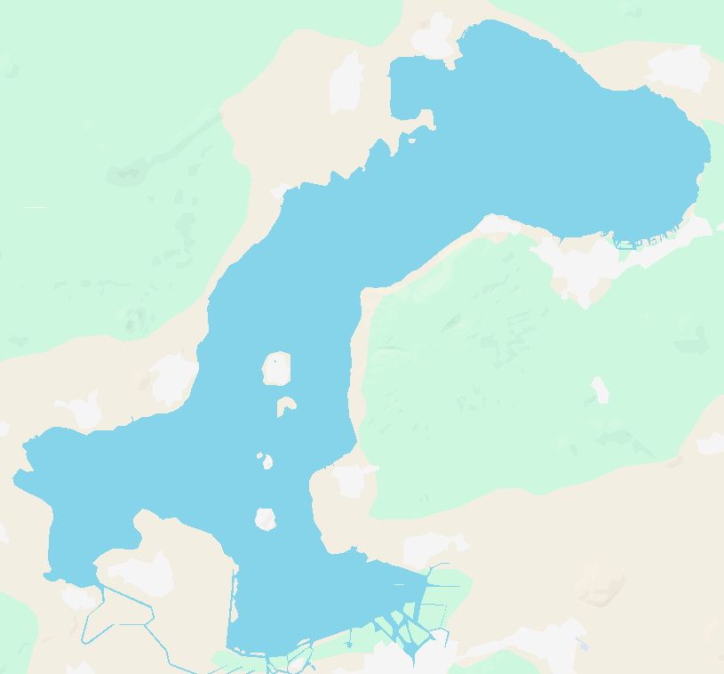
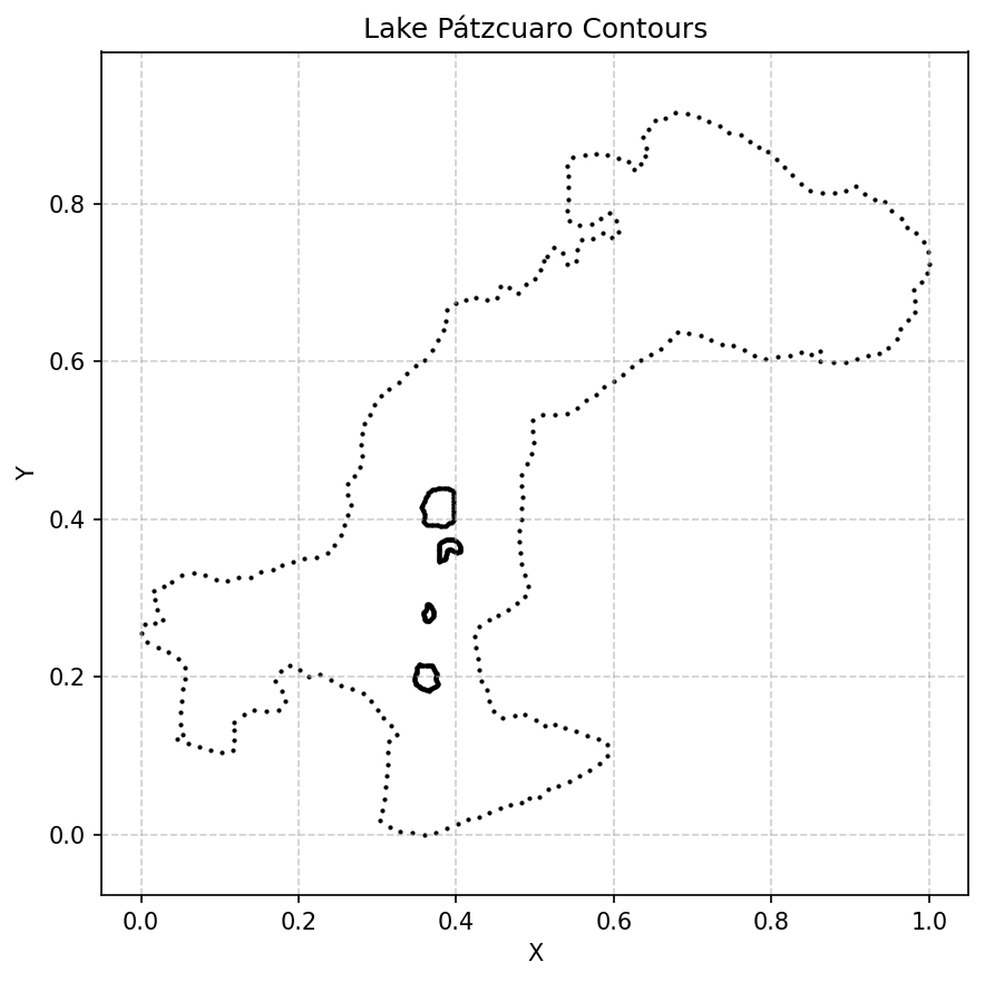
Instead of relying on idealized geometric shapes (circles or squares), mGFD excels at real geographic domains. We begin by identifying our domain boundaries from a satellite map and extracting the contours into a CSV file (Patzcuaro_contours.csv).
| Satellite Map | Extracted Contours (CSV Plot) |
 |
 |
Step 2: Generate the Cloud (CLI)
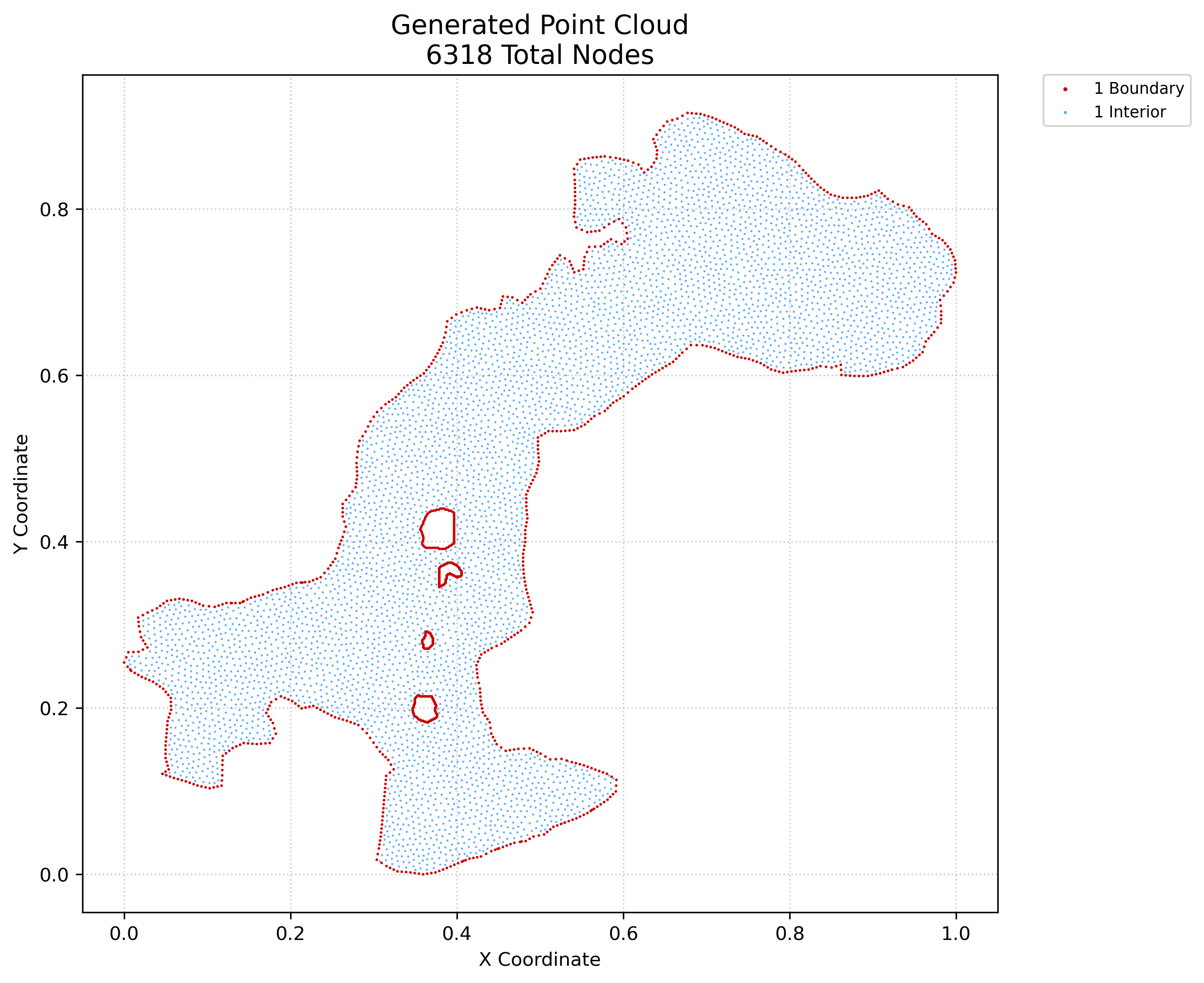
Using the built-in mgfd-cloud CLI, we fill the interior of the contour with an unstructured Poisson-Disk distributed point cloud:
mgfd-cloud generate --input Patzcuaro_contours.csv --output Patzcuaro_cloud.csv --method natural --density 3
Step 3: Python Solution
Option A: Modern Object-Oriented Interface (Recommended)
import numpy as np
from mGFD import Cloud, Domain, Dirichlet, PDE, Solver

# 1. Load point cloud geometry and compute local star stencils
cloud = Cloud.from_csv("Patzcuaro_cloud.csv", nvec=12)

# 2. Define Dirichlet boundary conditions (Callables, Floats, or Arrays)
bc = Dirichlet(lambda x, y: np.exp(x + y))
domain = Domain(cloud, boundary=bc)

# 3. Define the PDE physics: Stationary Poisson (order=0)
# Operator [D, E, 2*A, B, 2*C, F] -> Laplacian: [0, 0, 2, 0, 2, 0]
pde = PDE(
    operator=[0, 0, 2, 0, 2, 0],
    f=lambda x, y: 2 * np.exp(x + y),
    order=0,
    name="Pátzcuaro Poisson"
)

# 4. Configure and execute solver (supports CPU or CUDA)
solver = Solver(domain, pde, device="cpu", linear_solver="spsolve", verbose=True)
result = solver.solve()

# 5. One-line VTK export (ParaView) & 3D Matplotlib visualization
result.export_vtk("Patzcuaro_Poisson.vtu")
result.plot(title="Lake Pátzcuaro Poisson Solution")
Option B: Classic Functional Interface
import numpy as np
from mGFD.io.io import load_points
from mGFD.solvers import Stationary
from mGFD.viz.graph import plot_stationary

# 1. Load point cloud array [x, y, flag]
p = load_points("Patzcuaro_cloud.csv")

# 2. Define boundary and forcing functions
phi = lambda x, y: np.exp(x + y)
f_stat = lambda x, y: 2 * np.exp(x + y)
L_stat = [0, 0, 2, 0, 2, 0]

# 3. Solve Poisson equation
res = Stationary(p, phi, f_stat, operator=L_stat, linear_solver="spsolve", verbose=True)

# 4. Render 3D surface
plot_stationary(p, res.solution, title="Lake Pátzcuaro Poisson Solution", verbose=True)
Step 4: Visualize Results
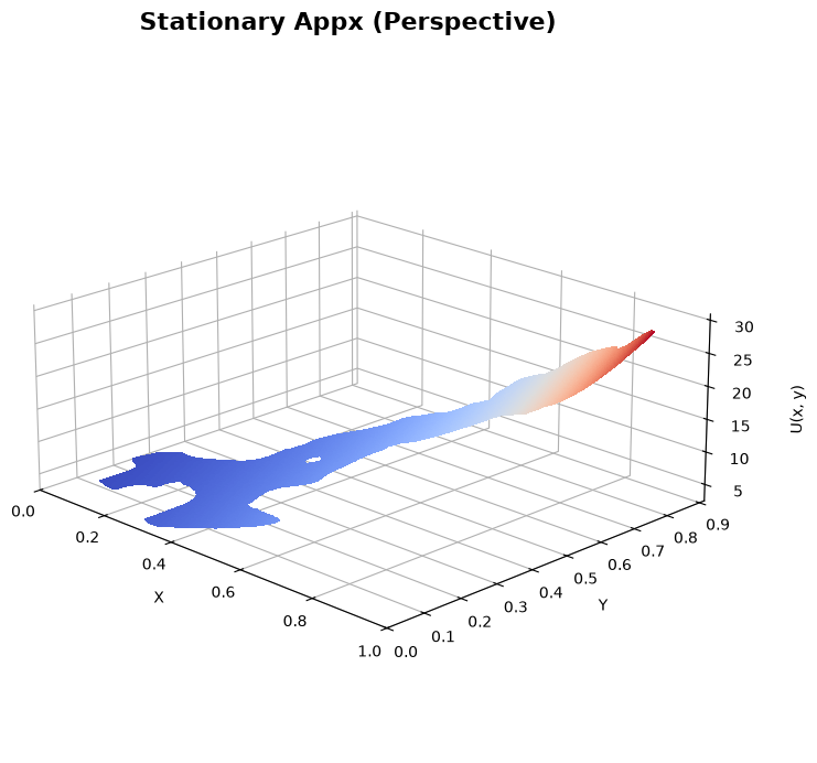
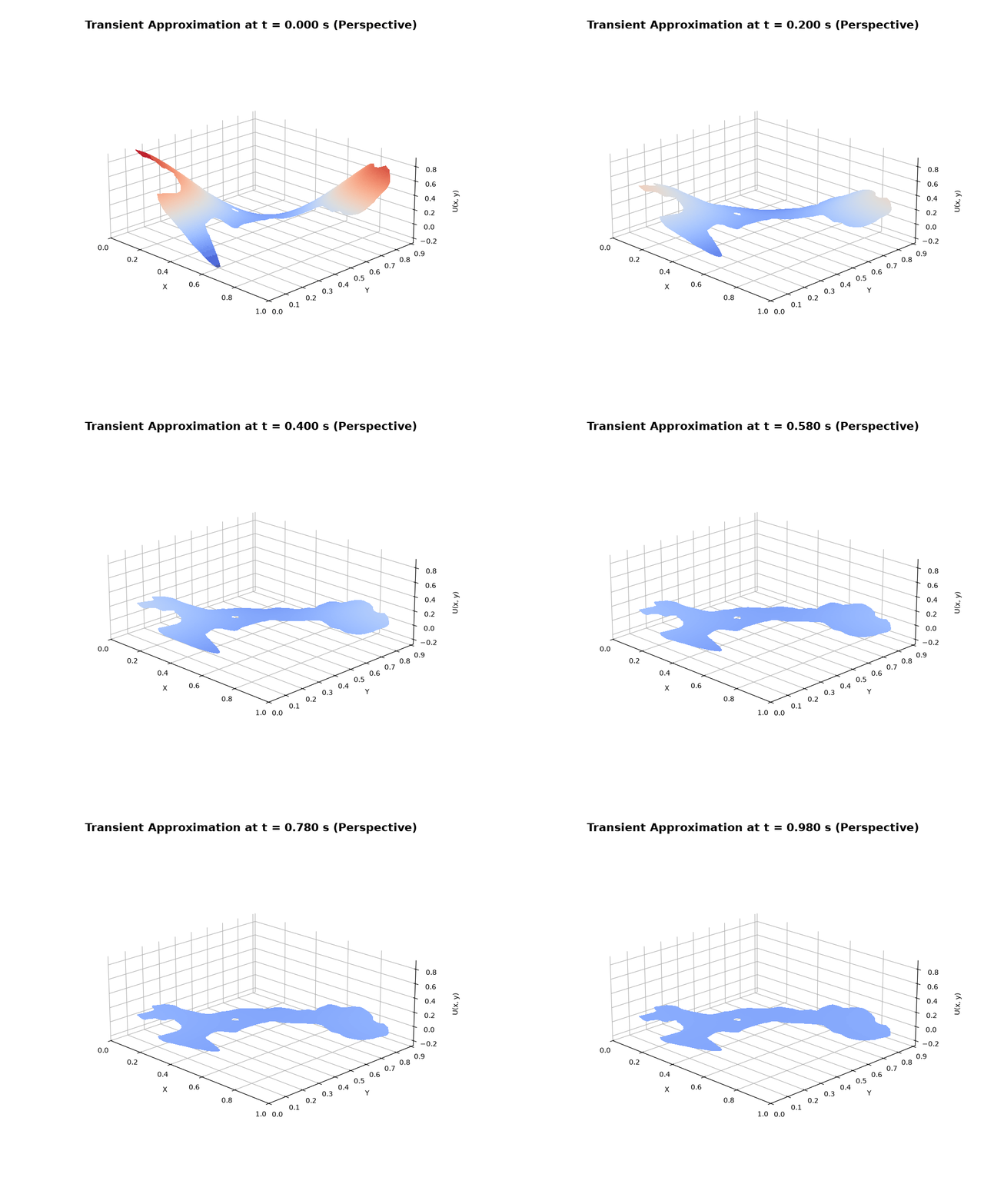
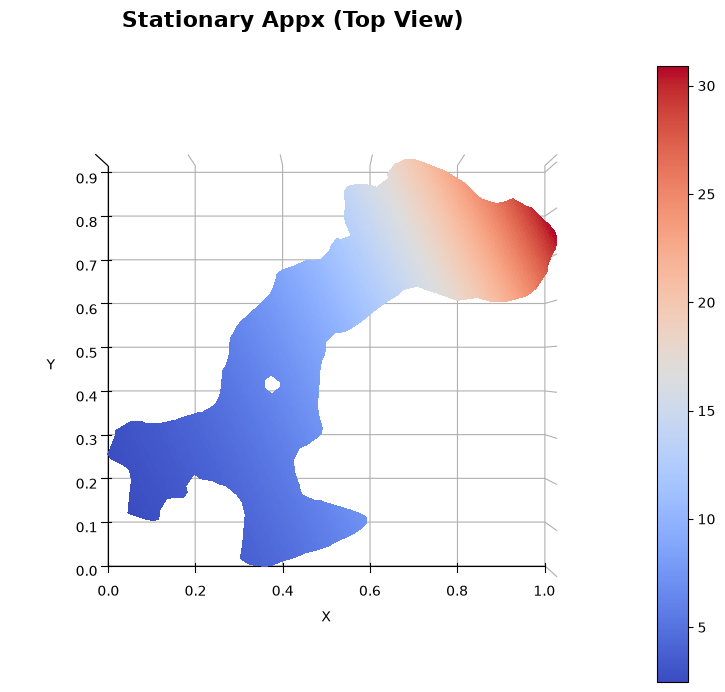
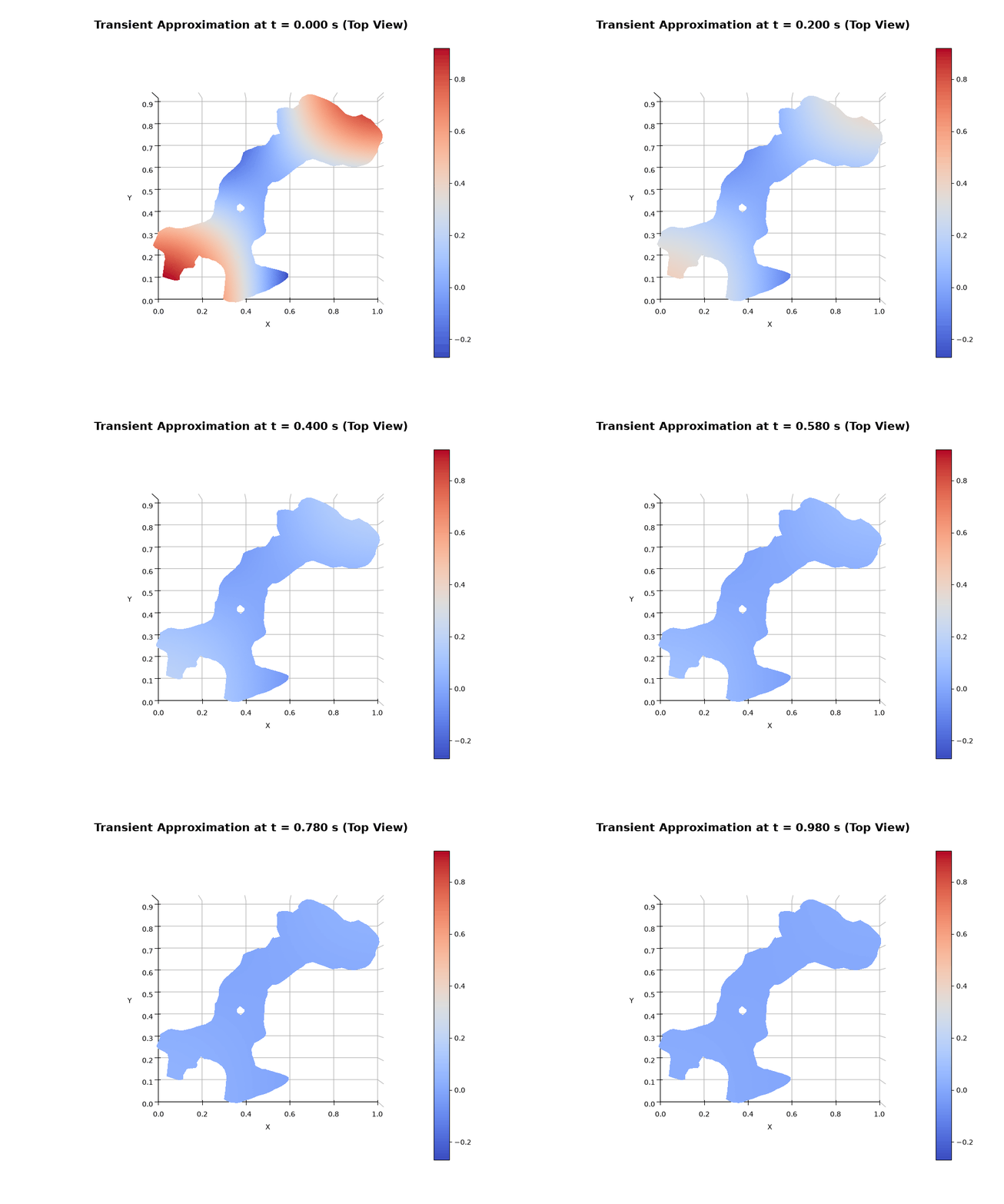
When running simulations or setting save=True, mGFD automatically exports publication-quality PNG snapshots (for stationary problems) and animated GIFs / MP4s (for transient problems).
| Poisson (Stationary) | Heat (Transient) |
 |
 |
 |
 |
📚 Python API Reference
mGFD provides both an intuitive, modern Object-Oriented interface (mGFD.oop) and a high-performance functional API (mGFD.solvers).
1. Modern Object-Oriented Interface (mGFD.oop)
The OOP interface organizes meshless modeling into clear abstractions: geometry (Cloud), boundaries (BoundaryCondition), domain integration (Domain), physics definition (PDE), solver execution (Solver), and results analysis (SolverResult).
Cloud
Encapsulates point cloud geometry, boundary classification flags, local characteristic lengths, and neighbor stencils.
class Cloud:
    def __init__(self, points: np.ndarray, nvec: int = 12, method: str = "natural") -> None
- Factory Methods:
Cloud.from_csv(file_path: str, nvec: int = 12, method: str = "natural") -> Cloud: Loads a cloud from CSV (x, y, flag).Cloud.from_array(points: np.ndarray, nvec: int = 12, method: str = "natural") -> Cloud: Instantiates from an(m, 3)NumPy array.Cloud.generate_natural(csv_file: str, density: float = 3.0, nvec: int = 12, inside_regions: bool = False, show: bool = False) -> Cloud: Generates a Poisson-Disk point cloud directly from a contour file.Cloud.generate_regular(csv_file: str, density: float = 3.0, nvec: int = 12, inside_regions: bool = False, show: bool = False) -> Cloud: Generates a regular grid point cloud from a contour file.
- Key Properties:
.points:(m, 3)NumPy array containing[x, y, flag]..n_points: Total number of nodes $m$..n_boundary/.n_interior: Number of boundary ($flag=1$) and interior ($flag=0$) nodes..boun_idx/.inne_idx: Integer indices of boundary and interior nodes..h_char,.h_min,.h_avg: Characteristic, minimum, and average node spacings..neighbors:(m, nvec)neighbor connectivity stencil matrix..valid_triangles: Cached Delaunay simplices for ParaView and Matplotlib visualization.
- Methods:
compute_neighbors(nvec: int = 12) -> np.ndarray: Computes spatial star stencils.set_boundary(boundary: BoundaryCondition) -> Domain: Pairs the cloud with a boundary condition to form aDomain.
BoundaryCondition (Dirichlet and Neumann)
Specifies physical boundary conditions across domain contours:
# Homogeneous Dirichlet (fixed boundary)
bc = Dirichlet(val=0.0)

# Spatially varying Dirichlet boundary condition
bc = Dirichlet(lambda x, y: np.sin(np.pi * x) * np.sin(np.pi * y))

# Time-dependent spatiotemporal Dirichlet boundary condition
bc = Dirichlet(lambda x, y, t: np.sin(x) * np.cos(t))

# Neumann boundary condition (flux du/dn)
bc = Neumann(val=0.0)
Domain
Integrates a Cloud geometry with a BoundaryCondition:
domain = Domain(cloud=cloud, boundary=bc)
# or fluently from the cloud:
domain = cloud.set_boundary(bc)
PDE
Defines arbitrary second-order linear physics without rigid equation-specific subclasses:
class PDE:
    def __init__(
        self,
        operator: Union[List[float], np.ndarray],
        f: Optional[Union[Callable, np.ndarray, float]] = None,
        order: int = 0,
        source: Optional[Union[Callable, np.ndarray, float]] = None,
        ic: Optional[Union[Callable, np.ndarray, float]] = None,
        g: Optional[Union[Callable, np.ndarray, float]] = None,
        name: str = "PDE"
    ) -> None
order: int: Temporal derivative order:0: Stationary ($L u = f(x, y)$)1: First-Order Transient ($\partial u / \partial t = L u + F_{\text{source}}(x, y, t)$)2: Second-Order Transient ($\partial^2 u / \partial t^2 = L u + F_{\text{source}}(x, y, t)$)
operator: 6-element vector[D, E, 2*A, B, 2*C, F]defining the spatial operator $L u = A u_{xx} + B u_{xy} + C u_{yy} + D u_x + E u_y + F u$.f: Analytical forcing function or boundary profile fallback.source: Non-homogeneous source term $F_{\text{source}}(x, y, t)$ (scalar, callable, or array).ic: Initial condition state $u_0(x, y)$ at $t = t_{\text{start}}$.g: Initial velocity profile $u_t(x, y)$ at $t = t_{\text{start}}$ (fororder=2wave equations).
Solver
The unified execution engine orchestrating CPU and CUDA solver backends:
solver = Solver(
    domain: Domain,
    pde: PDE,
    device: str = "cpu",                  # "cpu" or "cuda"
    linear_solver: str = "spsolve",       # "spsolve", "bicgstab", "gmres"
    matrix_free: bool = False,            # Memory-efficient matrix-free CPU solve
    preconditioner: Optional[str] = None, # "ilu" or "jacobi"
    symmetric: bool = True,               # Conservative Laplacian symmetrization (wave stability)
    alpha: float = 0.0,                   # HHT-alpha numerical damping [-0.333, 0.0]
    damping: float = 0.0,                 # Physical/numerical velocity damping (eta * u_t)
    upwind: Optional[bool] = None,        # Upwind neighbor weighting (default False for wave)
    verbose: bool = True
)

result: SolverResult = solver.solve(
    t_span: Tuple[float, float] = (0.0, 1.0),
    cfl: Optional[float] = 0.5,
    dt: Optional[float] = None,
    t_steps: Optional[int] = None,
    implicit: bool = True,
    lam: float = 0.5
)
SolverResult
A standardized container for PDE solution fields and execution telemetry:
- Attributes:
.solution: 1D array of shape(m,)(for stationary) or 2D array of shape(m, t)(for transients)..execution_time: Total wall-clock solve time in seconds..cfl: Courant-Friedrichs-Lewy number utilized during time-stepping..dt: Time step size $\Delta t$..t_steps: Number of computed temporal time steps..device: Device used ("cpu"or"cuda")..linear_solver: Linear algebra algorithm utilized.
- Methods:
.export_vtk(filename: str, out_dir: str = "."): Exports directly to ParaView.vtuformat..plot(save: bool = False, show: bool = True, nom: str = "", title: str = "Solution"): Automatically renders 3D surface plots or transient animations.- Tuple unpacking support:
u_ap, vec = resultis fully backward-compatible.
2. Classic Functional Solvers (mGFD.solvers)
The low-level functional API remains fully supported for backward compatibility and script-based pipelines.
Stationary
Solves stationary boundary-value problems (e.g., Poisson equation).
def Stationary(
    p: np.ndarray,
    phi: Union[Callable, np.ndarray, float],
    f: Union[Callable, np.ndarray, float],
    operator: Union[List[float], np.ndarray],
    upwind: bool = False,
    vec: Optional[np.ndarray] = None,
    nvec: int = 12,
    device: str = "cpu",
    linear_solver: str = "spsolve",
    matrix_free: bool = False,
    preconditioner: Optional[str] = None,
    verbose: bool = True
) -> SolverResult
TimeDerivative1
Solves first-order-in-time initial-boundary value problems (e.g., Heat and Advection-Diffusion equations).
def TimeDerivative1(
    p: np.ndarray,
    f: Optional[Union[Callable, np.ndarray, float]] = None,
    t: Optional[int] = None,
    coef: List[float] = [1.0],
    operator: Optional[Union[List[float], np.ndarray]] = None,
    implicit: bool = False,
    lam: float = 0.5,
    upwind: bool = False,
    vec: Optional[np.ndarray] = None,
    nvec: int = 12,
    device: str = "cpu",
    linear_solver: str = "spsolve",
    preconditioner: Optional[str] = None,
    verbose: bool = True,
    cfl: Optional[float] = None,
    dt: Optional[float] = None,
    ic: Optional[Union[Callable, np.ndarray, float]] = None,
    bc: Optional[Union[Callable, np.ndarray, float]] = None,
    source: Optional[Union[Callable, np.ndarray, float]] = None,
    t_span: Tuple[float, float] = (0.0, 1.0)
) -> SolverResult
TimeDerivative2
Solves second-order-in-time wave and hyperbolic systems.
def TimeDerivative2(
    p: np.ndarray,
    f: Optional[Union[Callable, np.ndarray, float]] = None,
    g: Union[Callable, np.ndarray, float] = 0.0,
    t: Optional[int] = None,
    coef: List[float] = [1.0],
    operator: Optional[Union[List[float], np.ndarray]] = None,
    upwind: bool = False,
    vec: Optional[np.ndarray] = None,
    nvec: int = 12,
    implicit: bool = True,
    lam: float = 0.25,
    device: str = "cpu",
    linear_solver: str = "spsolve",
    preconditioner: Optional[str] = None,
    verbose: bool = True,
    cfl: Optional[float] = None,
    dt: Optional[float] = None,
    ic: Optional[Union[Callable, np.ndarray, float]] = None,
    bc: Optional[Union[Callable, np.ndarray, float]] = None,
    source: Optional[Union[Callable, np.ndarray, float]] = None,
    t_span: Tuple[float, float] = (0.0, 1.0),
    symmetric: bool = True,
    alpha: float = 0.0,
    damping: float = 0.0
) -> SolverResult
symmetric: bool = True: Activates conservative Laplacian symmetrization $K = K^T \le 0$ to guarantee unconditional wave stability on irregular point clouds.alpha: float = 0.0: Hilber-Hughes-Taylor numerical damping parameter ($\alpha \in [-0.333, 0.0]$) to suppress spurious high-frequency spatial noise.damping: float = 0.0: Physical/numerical velocity damping coefficient ($\eta u_t$).
3. Cloud Generation (mGFD.cloud_generator)
Command-Line Interface (mgfd-cloud)
The mGFD package includes an automated CLI tool for rapid generation and reduction of computational clouds:
mgfd-cloud generate -i INPUT.csv -o OUTPUT.csv -m {natural,regular} [-d DENSITY] [--inside-regions]
mgfd-cloud reduce -i INPUT.csv -o OUTPUT.csv -m MULTIPLIER
generate: Fills a boundary contour with computational nodes.-i/--input: Path to boundary CSV file.-o/--output: Path for generated point cloud CSV.-m/--method: Sampling method (naturalfor Poisson-Disk orregularfor Grid).-d/--density: Density multiplier (e.g.,1,2,3,4).--inside-regions: If present, internal closed boundaries are treated as solid islands (holes in the domain).
reduce: Down-samples an existing cloud by a spatial multiplier factor (-m).
Python Generation Functions
def generate_cloud_natural(
    csv_file: str,
    output_file: str,
    inside_regions: bool = False,
    verbose: bool = False,
    show: bool = False
) -> None

def generate_cloud_regular(
    csv_file: str,
    output_file: str,
    inside_regions: bool = False,
    verbose: bool = False,
    show: bool = False
) -> None
- Setting
show=Falseprevents Matplotlib from opening interactive GUI windows, enabling headless batch generation.
4. I/O Operations (mGFD.io.io)
load_points
def load_points(file_path: str, verbose: bool = False) -> np.ndarray
Reads a point cloud CSV file and returns an (m, 3) NumPy array [x, y, flag].
export_stationary_vtk / export_transient_vtk (mGFD.io.export_vtk)
Exports numerical solutions directly to VTK/VTU format for 3D visualization and post-processing in ParaView:
def export_stationary_vtk(
    p: np.ndarray,
    u_ap: np.ndarray,
    out_dir: str,
    basename: str = "Stationary_Solution",
    cloud_path: Optional[str] = None
) -> None

def export_transient_vtk(
    p: np.ndarray,
    u_ap: np.ndarray,
    t: int,
    T: np.ndarray,
    out_dir: str,
    basename: str = "Transient_Solution",
    cloud_path: Optional[str] = None
) -> None
5. Visualization Utilities (mGFD.viz.graph)
plot_stationary
def plot_stationary(
    p: np.ndarray,
    u: np.ndarray,
    save: bool = False,
    nom: str = '',
    title: str = 'Solution',
    verbose: bool = True
) -> None
Renders a 3D surface plot over the unstructured point cloud and optionally saves .png snapshots.
plot_transient
def plot_transient(
    p: np.ndarray,
    u: np.ndarray,
    save: bool = False,
    nom: str = '',
    title: str = 'Solution',
    verbose: bool = True
) -> None
Renders an animated 3D Matplotlib animation over time. When imageio-ffmpeg is installed, compilation is accelerated by multi-threaded FFmpeg binaries (~6x speedup).
6. Core Utilities & Triangulations (mGFD.core.utils)
Because mGFD is a strictly meshless numerical method, the PDE solvers operate entirely on unstructured points and local distance-based neighborhoods. Triangulations are never used during the mathematical solve.
However, rendering 3D surfaces in Matplotlib and exporting meshes to ParaView requires a valid triangulation to interpolate color across faces:
get_valid_triangulation
def get_valid_triangulation(p: np.ndarray, nom: Optional[str] = None) -> Optional[np.ndarray]
Computes a constrained Delaunay triangulation, aggressively filtering simplices that cross concave boundaries or intersect internal islands. Triangulation results are automatically cached in a _triangulation.csv file adjacent to the original cloud file, eliminating repeated Delaunay computation overhead in subsequent runs.
⚡ High Performance, GPU & Conservative Symmetrization Guide
1. Conservative Laplacian Symmetrization (symmetric=True)
On unstructured point clouds, standard nearest-neighbor stencils produce asymmetric directed graphs: node $j$ may be in the neighbor stencil of node $i$, but node $i$ may not be in the stencil of node $j$. In hyperbolic wave equations ($u_{tt} = c^2 \nabla^2 u$), this asymmetry introduces non-conservative skew-symmetric components that pump artificial numerical energy into high-frequency modes, leading to exponential instability on fine, irregular meshes.
mGFD resolves this with Conservative Laplacian Symmetrization:
$$ W_{\text{sym}} = \frac{1}{2}\left(W + W^T\right), \quad D_{ii} = -\sum_{j \ne i} W_{\text{sym}, ij}, \quad K = K^T \le 0 $$
- Strict Symmetry: $K = K^T$ guarantees that all discrete spatial eigenvalues are strictly real ($\text{Im}(\lambda) \equiv 0$).
- Negative Semi-Definiteness: Row-sum diagonal balance ensures $\lambda \le 0$, completely preventing anti-diffusion energy growth.
- Energy Conservation: Preserves discrete Hamiltonian energy, yielding unconditionally stable wave propagation across complex natural lake contours across all scales.
2. Numerical Damping (HHT-$\alpha$ & Velocity Damping)
For long-duration transient simulations, high-frequency spatial dispersion can be suppressed using:
- Hilber-Hughes-Taylor $\alpha$-scheme (
alpha): Setting $\alpha \in [-0.333, 0.0]$ introduces controlled numerical dissipation into high-frequency modes without degrading second-order physical accuracy. - Velocity Damping (
damping): Adds a physical or numerical drag term $\eta u_t$ to dissipate shock waves and reflect boundary reflections smoothly.
3. Matrix-Free Operations (CPU Optimization)
Standard linear solvers construct a global $M \times M$ sparse matrix. Storing this matrix for large point clouds (e.g., > 1,000,000 nodes) consumes significant RAM.
By setting matrix_free=True, mGFD completely bypasses global matrix assembly. Numba JIT-compiled parallel closures compute matrix-vector products ($K \cdot x$) directly on the fly from point coordinates.
# RAM-efficient matrix-free solve on CPU
res = Stationary(
    p, phi, f_stat, operator=L_stat,
    linear_solver="bicgstab",
    matrix_free=True,
    device="cpu"
)
4. GPU Acceleration (NVIDIA CUDA via CuPy)
If an NVIDIA GPU is available and cupy is installed, passing device="cuda" offloads the linear algebra resolution directly to GPU VRAM using native CUDA BiCGSTAB iterative sparse solvers with warm-start state propagation:
# GPU-accelerated transient solve
res = TimeDerivative1(
    p, f_func, operator=L_adv_diff,
    device="cuda",
    linear_solver="bicgstab",
    cfl=0.5
)
5. Preconditioners for Iterative Solvers
When solving ill-conditioned systems on irregular clouds with Krylov solvers (bicgstab, gmres), mGFD provides built-in preconditioners:
- Jacobi (
preconditioner="jacobi"): Fast diagonal scaling for CPU and GPU. - Incomplete LU (
preconditioner="ilu"): Robust sparse factorization for challenging problems.
🔬 Research Laboratory & Datasets
Looking for the complete mathematical derivations, 20 real-world geographic lake datasets (Lake Pátzcuaro, Lake Ness, Lake Baikal, Caspian Sea, etc.), or reproducible benchmarking suites?
👉 Explore the Research Laboratory (/research/README.md)
The research/ directory contains:
research/METHODOLOGY.md: In-depth mathematical formulation, Taylor expansions, stencils, and stability theorems.research/DATASETS.md: Complete geographic dataset documentation, node counts across 4 scales, and bounding boxes for all 20 lakes.research/RESULTS.md: Benchmarking results across stationary Poisson, transient Heat, 2D Wave, and Advection-Reaction-Diffusion equations.
🏗️ Repository Structure
mGFD/
├── docs/                     # Media assets for README (logos, workflow images)
├── src/mGFD/                 # The core Python library (published to PyPI)
│   ├── oop/                  # Object-Oriented API (Cloud, Domain, PDE, Solver)
│   ├── cloud_generator/      # Point cloud generation & CLI (mgfd-cloud)
│   ├── spatial/              # Spatial discretization: KDTree neighbors, stencils
│   ├── temporal/             # CFL time-stepping & temporal stability
│   ├── solvers/              # High-level solvers (Stationary, TD1, TD2)
│   │   └── _backends/        # CPU (SciPy/Numba) and CUDA (CuPy) engines
│   ├── io/                   # CSV and ParaView VTK import/export operations
│   ├── utils/                # Adapters and helper functions
│   └── viz/                  # Matplotlib 3D surfaces and animations
├── research/                 # Academic reproducible research suite
│   ├── codes/                # Batch benchmarking scripts & runners
│   ├── data/                 # 20 lake geometries across 4 scale levels
│   ├── results/              # Output GIFs, VTKs, PNGs, and metrics
│   └── README.md             # Research suite documentation
├── examples/                 # Interactive tutorials (Poisson, Heat, Wave, etc.)
└── tests/                    # Comprehensive CI/CD unit test suite
🏛️ Institutional Support & Funding
This software and its theoretical foundation were developed by the Universidad Michoacana de San Nicolás de Hidalgo (UMSNH) in collaboration with institutional research partners.
 Universidad Michoacana de San Nicolás de Hidalgo |
 Secretaría de Ciencia, Humanidades, Tecnología e Innovación (SECIHTI) |
 Aula CIMNE-Morelia |
 SIIIA-MATH: Soluciones de Ingeniería |
Authors & Core Developers
- Dr. Gerardo Tinoco-Guerrero (Universidad Michoacana de San Nicolás de Hidalgo) — gerardo.tinoco@umich.mx
- Dr. Francisco Javier Domínguez-Mota (Universidad Michoacana de San Nicolás de Hidalgo) — francisco.mota@umich.mx
- Dr. José Alberto Guzmán-Torres (Universidad Michoacana de San Nicolás de Hidalgo) — jose.alberto.guzman@umich.mx
🤝 Contributing & Citation
Contributing
We welcome contributions from the scientific computing, computational mathematics, and open-source communities!
- Fork the repository.
- Clone your fork locally and create a feature branch (
git checkout -b feature-new-capability). - Develop your feature adhering strictly to our PEP-8 conventions (including trailing inline
#comments aligned to column 136). - Test your changes (
pytest tests/). - Open a Pull Request!
Citation
This project is open-sourced under the MIT License.
If you use mGFD in your research, computational modeling, or academic publications, please cite the reference paper:
@article{tinoco2025mgfd,
  title={mGFD: A meshless generalized finite difference method},
  author={Tinoco-Guerrero, Gerardo and Domínguez-Mota, Francisco Javier and Guzmán-Torres, José Alberto and Pedraza-Jiménez, Gabriela and Tinoco-Ruiz, José Gerardo},
  journal={Computers & Mathematics with Applications},
  volume={195},
  pages={396--418},
  year={2025},
  publisher={Elsevier},
  doi={10.1016/j.camwa.2025.07.034}
}
Developed for the advancement of meshless numerical methods and scientific computing.
Report a Bug | Discussions | Contact Author
1 maintainer

Metadata
1 maintainer
Release files for mGFD 0.12.1
For a detailed explanation of source distributions (sdists) and built distributions (wheels), please see the package formats documentation.
Source distribution (sdist)
| File | Size | Uploaded | |
|---|---|---|---|
| mgfd-0.12.1.tar.gz | 158.4 kB | Details |
Built distribution (wheel)
| File | Interpreter | ABI | Platform | Reset |
|---|---|---|---|---|
| mgfd-0.12.1-py3-none-any.whl | Python 3 | none | any | Details |
Total release size: 332.3 kB
Release files / mgfd-0.12.1.tar.gz
| Download URL | mgfd-0.12.1.tar.gz |
|---|---|
| Size | 158.4 kB |
| Tags | Source |
|
SHA-256 checksum How to use checksums |
d258dfa9815ac16fc036ba1face943d8d49ac52501abd8bab677f82f98e5fa2c
|
|
BLAKE2b-256 checksum How to use checksums |
ea62d381fd259deb31e98a28244802cffc266e59a464ba294fb9e75e5992b892
|
| Upload date | |
|
Uploaded using Trusted Publishing? What is trusted publishing? |
No |
| Uploaded via |
twine/7.0.0 CPython/3.13.7
|
Release files / mgfd-0.12.1-py3-none-any.whl
| Download URL | mgfd-0.12.1-py3-none-any.whl |
|---|---|
| Size | 173.9 kB |
| Tags | Python 3 |
|
SHA-256 checksum How to use checksums |
83c0db0477d85fe2031fd03fb2202cae1e5ff831319759ca6e0f7fd91b448973
|
|
BLAKE2b-256 checksum How to use checksums |
fc4d49b7e656f2e612895e6c65b161f3405881057a427aa661d5cc2f49c4ff6f
|
| Upload date | |
|
Uploaded using Trusted Publishing? What is trusted publishing? |
No |
| Uploaded via |
twine/7.0.0 CPython/3.13.7
|














