Imputes missing data with MICE + random forests

Project description


miceforest: Fast Imputation with lightgbm in Python

Fast, memory efficient Multiple Imputation by Chained Equations (MICE) with random forests. It can impute categorical and numeric data without much setup, and has an array of diagnostic plots available. The R version of this package may be found here.
This document contains a thorough walkthrough of the package, benchmarks, and an introduction to multiple imputation. More information on MICE can be found in Stef van Buuren’s excellent online book, which you can find here.
Table of Contents:
Package Meta
miceforest has 4 main classes which the user will interact with:
KernelDataSet- a kernel data set is a dataset on which the mice algorithm is performed. Models are saved inside the instance, which can also be called on to impute new data. Several plotting methods are included to run diagnostics on the imputed data.MultipleImputedKernel- a collection ofKernelDataSets. Has additional methods for accessing and comparing multiple kernel datasets together.ImputedDataSet- a single dataset that has been imputed. These are returned afterimpute_new_data()is called.MultipleImputedDataSet- A collection of datasets that have been imputed. Has additional methods for comparing the imputations between datasets.
This package can be installed using either pip or conda, through conda-forge:
# Using pip
$ pip install miceforest

# Using conda
$ conda install -c conda-forge miceforest
You can also download the latest development version from this
repository. If you want to install from github with conda, you must
first run conda install pip git.
$ pip install git+https://github.com/AnotherSamWilson/miceforest.git
Using miceforest
We will be looking at a few simple examples of imputation. We need to load the packages, and define the data:
import miceforest as mf
from sklearn.datasets import load_iris
import pandas as pd
import numpy as np

# Load data and introduce missing values
iris = pd.concat(load_iris(as_frame=True,return_X_y=True),axis=1)
iris['target'] = iris['target'].astype('category')
iris_amp = mf.ampute_data(iris,perc=0.25,random_state=1991)
Imputing a Single Dataset
If you only want to create a single imputed dataset, you can use
KernelDataSet:
# Create kernel.
kds = mf.KernelDataSet(
  iris_amp,
  save_all_iterations=True,
  random_state=1991
)

# Run the MICE algorithm for 3 iterations
kds.mice(3)

# Return the completed kernel data
completed_data = kds.complete_data()
There are also an array of plotting functions available, these are discussed below in the section Diagnostic Plotting. The plotting behavior between single imputed datasets and multi-imputed datasets is slightly different.
Simple Example of Multiple Imputation
We can also create a class which contains multiple KernelDataSets,
along with easy ways to compare them:
# Create kernel.
kernel = mf.MultipleImputedKernel(
  iris_amp,
  datasets=4,
  save_all_iterations=True,
  random_state=1991
)

# Run the MICE algorithm for 3 iterations on each of the datasets
kernel.mice(3)
Printing the MultipleImputedKernel object will tell you some high
level information:
print(kernel)
##               Class: MultipleImputedKernel
##        Models Saved: Last Iteration
##            Datasets: 4
##          Iterations: 3
##   Imputed Variables: 5
## save_all_iterations: True
Controlling Tree Growth
Parameters can be passed directly to lightgbm in several different ways.
Parameters you wish to apply globally to every model can simply be
passed as kwargs to mice:
# Run the MICE algorithm for 2 more iterations on the kernel
kernel.mice(1,n_estimators=50)
You can also pass pass variable-specific arguments to
variable_parameters in mice. For instance, let’s say you noticed the
imputation of the [target] column was taking a little longer, because
it is multiclass. You could decrease the n_estimators specifically for
that column with:
# Run the MICE algorithm for 2 more iterations on the kernel
kernel.mice(1,variable_parameters={'target': {'n_estimators': 25}},n_estimators=50)
In this scenario, any parameters specified in variable_parameters
takes presidence over the kwargs.
Imputing with Gradient Boosted Trees
Since any arbitrary parameters can be passed to lightgbm.train(), it
is possible to change the algrorithm entirely. This can be done simply
like so:
# Create kernel.
kds_gbdt = mf.KernelDataSet(
  iris_amp,
  save_all_iterations=True,
  random_state=1991
)

# We need to add a minimum hessian, or lightgbm will complain:
kds_gbdt.mice(3, boosting='gbdt', min_sum_hessian_in_leaf=1)

# Return the completed kernel data
completed_data = kds_gbdt.complete_data()
Customizing the Imputation Process
It is possible to heavily customize our imputation procedure by
variable. By passing a named list to variable_schema, you can specify
the predictors for each variable to impute. You can also specify
mean_match_candidates and mean_match_subset by variable by passing a
dict of valid values, with variable names as keys. You can even replace
the entire default mean matching function if you wish:
var_sch = {
    'sepal width (cm)': ['target','petal width (cm)'],
    'petal width (cm)': ['target','sepal length (cm)']
}
var_mmc = {
    'sepal width (cm)': 5,
    'petal width (cm)': 0
}
var_mms = {
  'sepal width (cm)': 50
}

# The mean matching function requires these parameters, even
# if it does not use them.
def mmf(
        mmc,
        candidate_preds,
        bachelor_preds,
        candidate_values,
        cat_dtype,
        random_state):

    imp_values = random_state.choice(candidate_values, size=bachelor_preds.shape[0])
    if cat_dtype is not None:
        imp_values = cat_dtype.categories[imp_values]

    return imp_values

cust_kernel = mf.MultipleImputedKernel(
    iris_amp,
    datasets=3,
    variable_schema=var_sch,
    mean_match_candidates=var_mmc,
    mean_match_subset=var_mms,
    mean_match_function=mmf
)
cust_kernel.mice(2)
Imputing New Data with Existing Models
Multiple Imputation can take a long time. If you wish to impute a
dataset using the MICE algorithm, but don’t have time to train new
models, it is possible to impute new datasets using a
MultipleImputedKernel object. The impute_new_data() function uses
the random forests collected by MultipleImputedKernel to perform
multiple imputation without updating the random forest at each
iteration:
# Our 'new data' is just the first 15 rows of iris_amp
new_data = iris_amp.iloc[range(15)]
new_data_imputed = kernel.impute_new_data(new_data=new_data)
print(new_data_imputed)
##               Class: MultipleImputedDataSet
##            Datasets: 4
##          Iterations: 5
##   Imputed Variables: 5
## save_all_iterations: False
All of the imputation parameters (variable_schema,
mean_match_candidates, etc) will be carried over from the original
MultipleImputedKernel object. When mean matching, the candidate values
are pulled from the original kernel dataset. To impute new data, the
save_models parameter in MultipleImputedKernel must be > 0. If
save_models == 1, the model from the latest iteration is saved for
each variable. If save_models > 1, the model from each iteration is
saved. This allows for new data to be imputed in a more similar fashion
to the original mice procedure.
How to Make the Process Faster
Multiple Imputation is one of the most robust ways to handle missing data - but it can take a long time. There are several strategies you can use to decrease the time a process takes to run:
- Decrease
mean_match_subset. By default all non-missing datapoints are considered as candidates. This can cause the nearest-neighbors search to take a long time for large data. A subset of these points can be searched instead by usingmean_match_subset. - Decrease
mean_match_candidates. If your data is large, the default mean_match_candidates for each variable is 0.001 * (# non-missing datapoints). This can grow to be an unweidly large number of neighbors that need to be found. - Use different lightgbm parameters. lightgbm is usually not the problem, however if a certain variable has a large number of classes, then the max number of trees actually grown is (# classes) * (n_estimators). You can specifically decrease the bagging fraction or n_estimators for large multi-class variables.
- Use a faster mean matching function. The default mean matching function uses the sklearn.neighbors.NearestNeighbors algorithm. There are faster alternatives out there (faiss), however faiss is only available from conda.
Diagnostic Plotting
As of now, miceforest has four diagnostic plots available.
Distribution of Imputed-Values
We probably want to know how the imputed values are distributed. We can
plot the original distribution beside the imputed distributions in each
dataset by using the plot_imputed_distributions method of an
MultipleImputedKernel object:
kernel.plot_imputed_distributions(wspace=0.3,hspace=0.3)
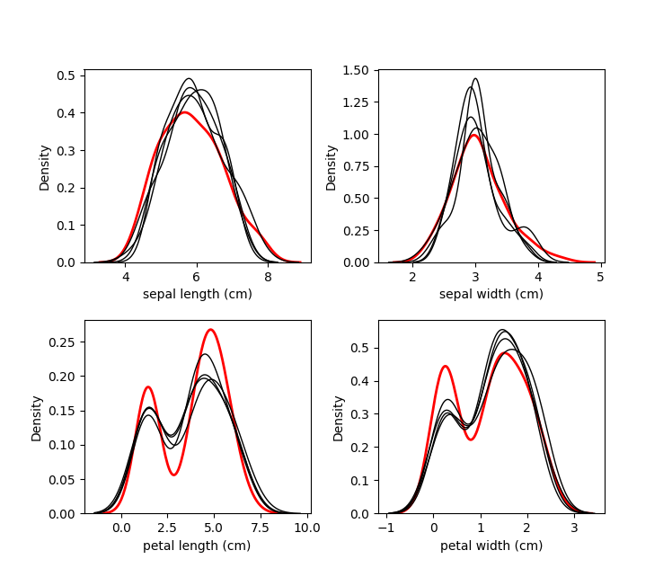
The red line is the original data, and each black line are the imputed values of each dataset.
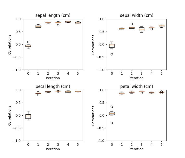
Convergence of Correlation
We are probably interested in knowing how our values between datasets
converged over the iterations. The plot_correlations method shows you
a boxplot of the correlations between imputed values in every
combination of datasets, at each iteration. This allows you to see how
correlated the imputations are between datasets, as well as the
convergence over iterations:
kernel.plot_correlations()
Variable Importance
We also may be interested in which variables were used to impute each
variable. We can plot this information by using the
plot_feature_importance method.
kernel.plot_feature_importance(annot=True,cmap="YlGnBu",vmin=0, vmax=1)
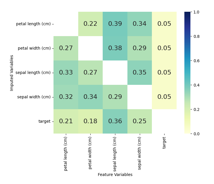
The numbers shown are returned from the
lightgbm.Booster.feature_importance() function. Each square represents
the importance of the column variable in imputing the row variable.
Mean Convergence
If our data is not missing completely at random, we may see that it takes a few iterations for our models to get the distribution of imputations right. We can plot the average value of our imputations to see if this is occurring:
kernel.plot_mean_convergence(wspace=0.3, hspace=0.4)
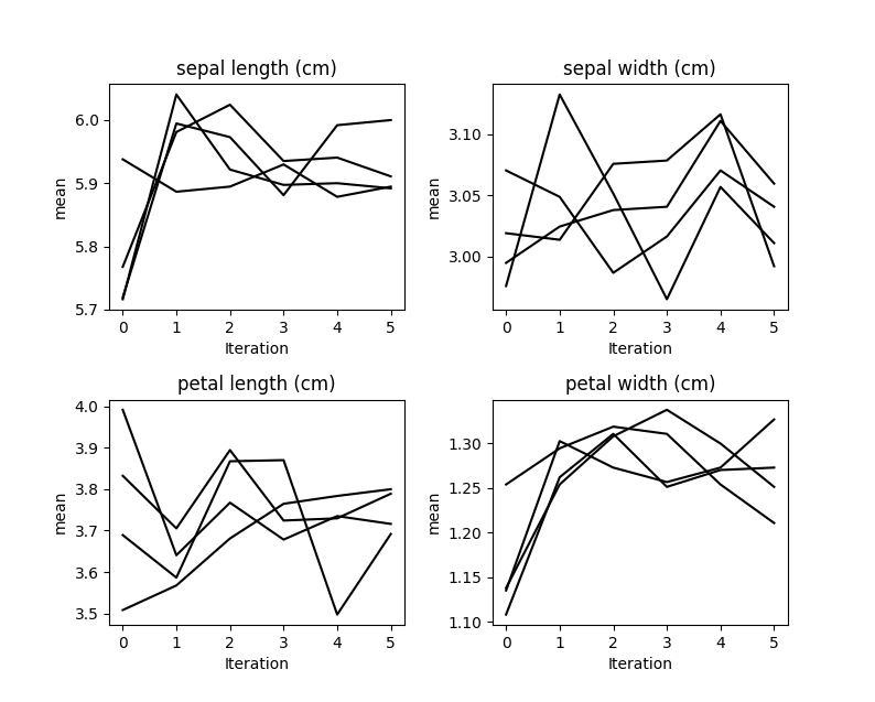
Our data was missing completely at random, so we don’t see any convergence occurring here.
Using the Imputed Data
To return the imputed data simply use the complete_data method:
dataset_1 = kernel.complete_data(0)
This will return a single specified dataset. Multiple datasets are typically created so that some measure of confidence around each prediction can be created.
Since we know what the original data looked like, we can cheat and see how well the imputations compare to the original data:
acclist = []
for iteration in range(kernel.iteration_count()+1):
    target_na_count = kernel.na_counts['target']
    compdat = kernel.complete_data(dataset=0,iteration=iteration)

    # Record the accuract of the imputations of target.
    acclist.append(
      round(1-sum(compdat['target'] != iris['target'])/target_na_count,2)
    )

# acclist shows the accuracy of the imputations
# over the iterations.
print(acclist)
## [0.32, 0.84, 0.81, 0.68, 0.81, 0.86]
In this instance, we went from a ~32% accuracy (which is expected with random sampling) to an accuracy of ~86% after the first iteration. The accuracy kind of floundered around afterwards. This is typical when the data is Missing Completely At Random. If the data were more Missing At Random, we might see a more normal convergence of accuracy.
The MICE Algorithm
Multiple Imputation by Chained Equations ‘fills in’ (imputes) missing data in a dataset through an iterative series of predictive models. In each iteration, each specified variable in the dataset is imputed using the other variables in the dataset. These iterations should be run until it appears that convergence has been met.
This process is continued until all specified variables have been imputed. Additional iterations can be run if it appears that the average imputed values have not converged, although no more than 5 iterations are usually necessary.
Common Use Cases
Data Leakage:
MICE is particularly useful if missing values are associated with the target variable in a way that introduces leakage. For instance, let’s say you wanted to model customer retention at the time of sign up. A certain variable is collected at sign up or 1 month after sign up. The absence of that variable is a data leak, since it tells you that the customer did not retain for 1 month.
Funnel Analysis:
Information is often collected at different stages of a ‘funnel’. MICE can be used to make educated guesses about the characteristics of entities at different points in a funnel.
Confidence Intervals:
MICE can be used to impute missing values, however it is important to keep in mind that these imputed values are a prediction. Creating multiple datasets with different imputed values allows you to do two types of inference:
- Imputed Value Distribution: A profile can be built for each imputed value, allowing you to make statements about the likely distribution of that value.
- Model Prediction Distribution: With multiple datasets, you can build multiple models and create a distribution of predictions for each sample. Those samples with imputed values which were not able to be imputed with much confidence would have a larger variance in their predictions.
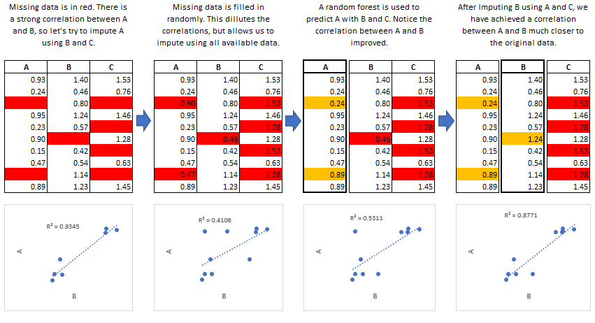
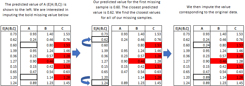
Predictive Mean Matching
miceforest can make use of a procedure called predictive mean matching
(PMM) to select which values are imputed. PMM involves selecting a
datapoint from the original, nonmissing data which has a predicted value
close to the predicted value of the missing sample. The closest N
(mean_match_candidates parameter) values are chosen as candidates,
from which a value is chosen at random. This can be specified on a
column-by-column basis. Going into more detail from our example above,
we see how this works in practice:
This method is very useful if you have a variable which needs imputing which has any of the following characteristics:
- Multimodal
- Integer
- Skewed
Effects of Mean Matching
As an example, let’s construct a dataset with some of the above characteristics:
randst = np.random.RandomState(1991)
# random uniform variable
nrws = 1000
uniform_vec = randst.uniform(size=nrws)

def make_bimodal(mean1,mean2,size):
    bimodal_1 = randst.normal(size=nrws, loc=mean1)
    bimodal_2 = randst.normal(size=nrws, loc=mean2)
    bimdvec = []
    for i in range(size):
        bimdvec.append(randst.choice([bimodal_1[i], bimodal_2[i]]))
    return np.array(bimdvec)

# Make 2 Bimodal Variables
close_bimodal_vec = make_bimodal(2,-2,nrws)
far_bimodal_vec = make_bimodal(3,-3,nrws)


# Highly skewed variable correlated with Uniform_Variable
skewed_vec = np.exp(uniform_vec*randst.uniform(size=nrws)*3) + randst.uniform(size=nrws)*3

# Integer variable correlated with Close_Bimodal_Variable and Uniform_Variable
integer_vec = np.round(uniform_vec + close_bimodal_vec/3 + randst.uniform(size=nrws)*2)

# Make a DataFrame
dat = pd.DataFrame(
    {
    'uniform_var':uniform_vec,
    'close_bimodal_var':close_bimodal_vec,
    'far_bimodal_var':far_bimodal_vec,
    'skewed_var':skewed_vec,
    'integer_var':integer_vec
    }
)

# Ampute the data.
ampdat = mf.ampute_data(dat,perc=0.25,random_state=randst)

# Plot the original data
import seaborn as sns
import matplotlib.pyplot as plt
g = sns.PairGrid(dat)
g.map(plt.scatter,s=5)
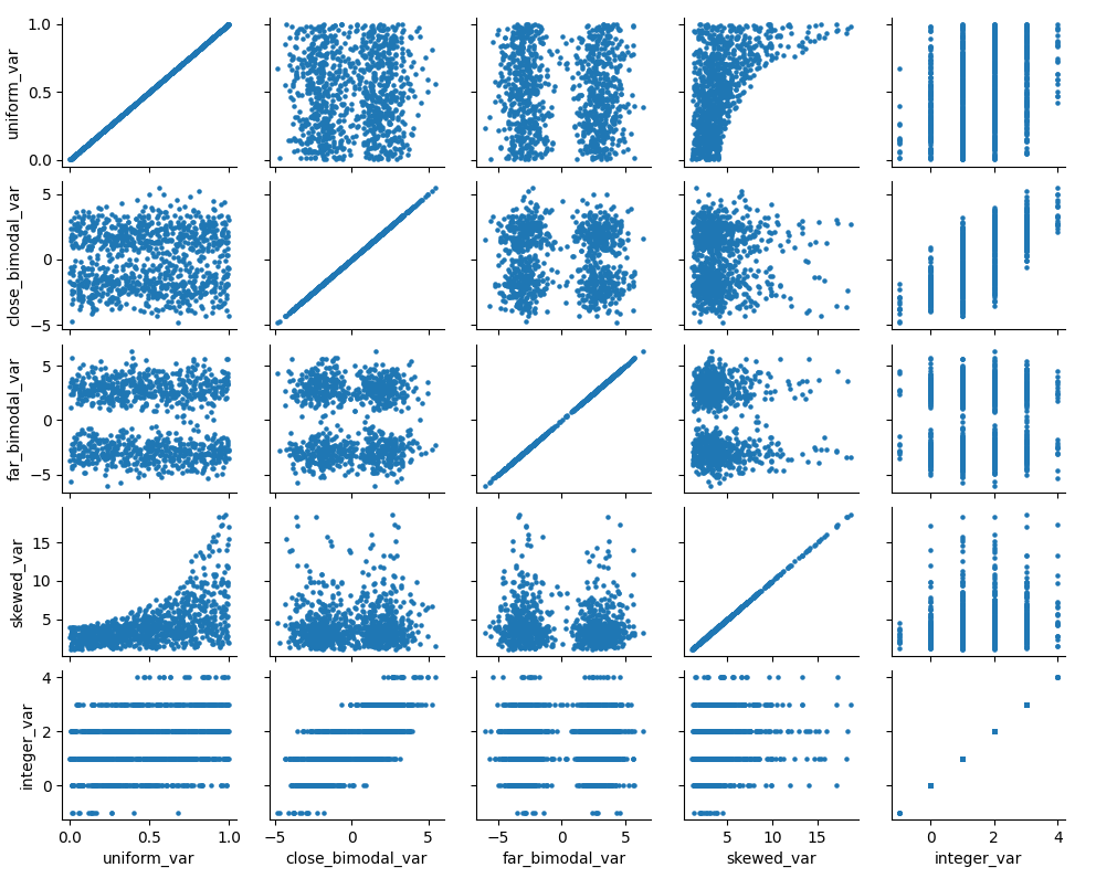 We can see how our variables are distributed and correlated in the graph
above. Now let’s run our imputation process twice, once using mean
matching, and once using the model prediction.
We can see how our variables are distributed and correlated in the graph
above. Now let’s run our imputation process twice, once using mean
matching, and once using the model prediction.
kernelmeanmatch <- mf.MultipleImputedKernel(ampdat,mean_match_candidates=5)
kernelmodeloutput <- mf.MultipleImputedKernel(ampdat,mean_match_candidates=0)

kernelmeanmatch.mice(5)
kernelmodeloutput.mice(5)
Let’s look at the effect on the different variables.
With Mean Matching
kernelmeanmatch.plot_imputed_distributions(wspace=0.2,hspace=0.4)
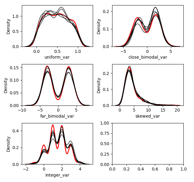
Without Mean Matching
kernelmodeloutput.plot_imputed_distributions(wspace=0.2,hspace=0.4)
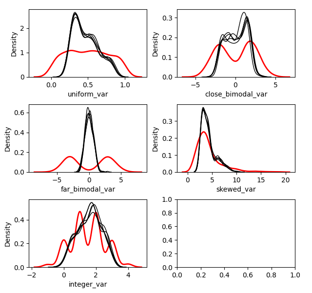
You can see the effects that mean matching has, depending on the distribution of the data. Simply returning the value from the model prediction, while it may provide a better ‘fit’, will not provide imputations with a similair distribution to the original. This may be beneficial, depending on your goal.
Release history Release notifications | RSS feed


Download files
Download the file for your platform. If you're not sure which to choose, learn more about installing packages.
Source Distribution
Built Distribution
Filter files by name, interpreter, ABI, and platform.
If you're not sure about the file name format, learn more about wheel file names.
Copy a direct link to the current filters
File details
Details for the file miceforest-3.0.1.tar.gz.
File metadata
- Download URL: miceforest-3.0.1.tar.gz
- Upload date:
- Size: 37.2 kB
- Tags: Source
- Uploaded using Trusted Publishing? No
- Uploaded via: twine/3.4.2 importlib_metadata/4.8.1 pkginfo/1.7.1 requests/2.26.0 requests-toolbelt/0.9.1 tqdm/4.62.2 CPython/3.9.6
File hashes
| Algorithm | Hash digest | |
|---|---|---|
| SHA256 |
387d16745aeaa1ad3d34d9d02995acc74787396c813ce8ebbea3901a80617bcc
|
|
| MD5 |
aca5b5f355adaa96e08a353959c8b6ee
|
|
| BLAKE2b-256 |
00b5d8f4df56135a6e2e0f0985543fc7855eede3da859b54a066a39d14ddbaa6
|
File details
Details for the file miceforest-3.0.1-py3-none-any.whl.
File metadata
- Download URL: miceforest-3.0.1-py3-none-any.whl
- Upload date:
- Size: 31.8 kB
- Tags: Python 3
- Uploaded using Trusted Publishing? No
- Uploaded via: twine/3.4.2 importlib_metadata/4.8.1 pkginfo/1.7.1 requests/2.26.0 requests-toolbelt/0.9.1 tqdm/4.62.2 CPython/3.9.6
File hashes
| Algorithm | Hash digest | |
|---|---|---|
| SHA256 |
ac886112aee519535f3dc24139be56cf2345e34d2d5ab3250fef6cc69d540087
|
|
| MD5 |
1e1e8ad4e63c03986fa67df54e764f97
|
|
| BLAKE2b-256 |
34f0fe7d7776d9db262bfba7d9d96e8803f3a098cb60dc4efe8816e1ed6dd7ec
|


