
MicroKeras

MicroKeras is a minimal implementation of the Sequential Class from the Keras deep-learning library, built from scratch using Python and NumPy. It provides a simple and intuitive API for building, training, and evaluating neural networks inspired by the Keras API.
Documentation
For full documentation, please visit https://microkeras.readthedocs.io/en/latest/
Installation
To install MicroKeras, use pip:
pip install microkeras
Features
MicroKeras offers the following features:
- Sequential model API
- Dense (fully connected) layers
- Various activation functions (ReLU, Sigmoid, Softmax, Linear)
- Loss functions (Mean Squared Error, Categorical Cross-Entropy)
- Optimizers (Stochastic Gradient Descent)
- Dataset loaders (MNIST, California Housing)
- Model saving and loading
Quick Start: MNIST Classification Example
Let's walk through a complete example using MicroKeras to classify handwritten digits from the MNIST dataset. This example will demonstrate how to load data, create a model, train it, make predictions, and save/load the model.
Importing Dependencies
First, let's import the necessary modules:
import numpy as np
from microkeras.models import Sequential
from microkeras.layers import Dense
from microkeras.optimizers import SGD
from microkeras.datasets import mnist
Loading and Preprocessing Data
Next, we'll load the MNIST dataset and preprocess it:
# Load and preprocess MNIST data
(X_train, y_train), (X_test, y_test) = mnist.load_data()

# Reshape and normalize the input data
X_train = X_train.reshape(X_train.shape[0], -1)
X_test = X_test.reshape(X_test.shape[0], -1)

# One-hot encode the labels
y_train = np.eye(10)[y_train]
y_test = np.eye(10)[y_test]

print("Data shapes:")
print(f"X_train: {X_train.shape}, y_train: {y_train.shape}")
print(f"X_test: {X_test.shape}, y_test: {y_test.shape}")
Output:
Data shapes:
X_train: (56000, 784), y_train: (56000, 10)
X_test: (14000, 784), y_test: (14000, 10)
Creating the Model
Now, let's create our Sequential model:
model = Sequential([
    Dense(200, activation='sigmoid', input_shape=(784,)),
    Dense(200, activation='sigmoid'),
    Dense(10, activation='softmax')
])
This model consists of two hidden layers with sigmoid activation and an output layer with softmax activation, suitable for multi-class classification.
Compiling the Model
We'll compile the model using Stochastic Gradient Descent (SGD) as the optimizer and Categorical Cross-Entropy as the loss function:
optimizer = SGD(learning_rate=0.1)
model.compile(optimizer=optimizer,
              loss='categorical_crossentropy',
              metrics=['accuracy'])
Training the Model
Let's train the model for 10 epochs with a batch size of 32:
history = model.fit(X_train,
                    y_train,
                    batch_size=16,
                    epochs=10)
Output:
Epoch 1/10
Batch 3500/3500 - Loss: 4.9410, Acc: 0.9238: : 3712it [00:37, 99.54it/s]
Epoch 2/10
Batch 3500/3500 - Loss: 1.9095, Acc: 0.9746: : 3712it [00:20, 180.73it/s]
Epoch 3/10
Batch 3500/3500 - Loss: 1.5755, Acc: 0.9844: : 3712it [00:21, 168.76it/s]
Epoch 4/10
Batch 3500/3500 - Loss: 1.2145, Acc: 0.9844: : 3712it [00:22, 162.42it/s]
Epoch 5/10
Batch 3500/3500 - Loss: 0.9108, Acc: 0.9902: : 3712it [00:23, 157.83it/s]
Epoch 6/10
Batch 3500/3500 - Loss: 0.7050, Acc: 0.9941: : 3712it [00:21, 175.94it/s]
Epoch 7/10
Batch 3500/3500 - Loss: 0.4757, Acc: 0.9980: : 3712it [00:20, 183.64it/s]
Epoch 8/10
Batch 3500/3500 - Loss: 0.4843, Acc: 1.0000: : 3712it [00:22, 164.84it/s]
Epoch 9/10
Batch 3500/3500 - Loss: 0.4095, Acc: 0.9980: : 3712it [00:22, 164.12it/s]
Epoch 10/10
Batch 3500/3500 - Loss: 0.3842, Acc: 0.9961: : 3712it [00:21, 176.15it/s]
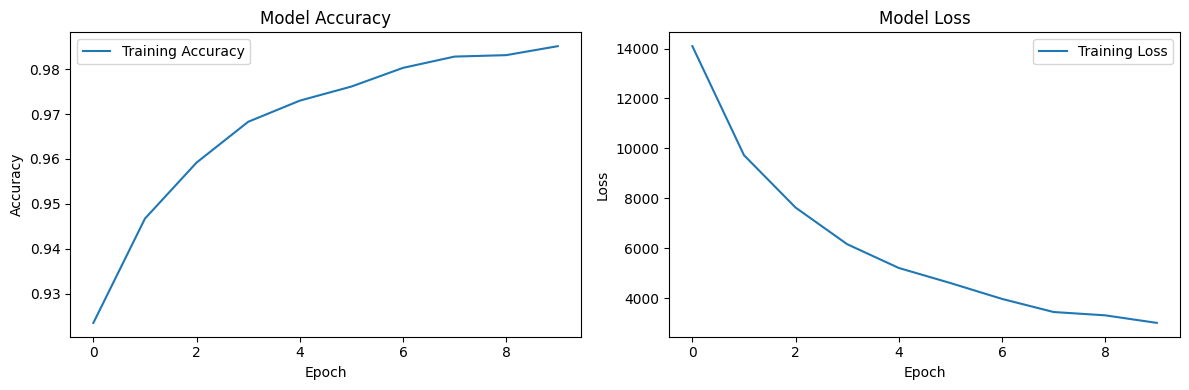
Plotting Training History
We can plot the training history using Matplotlib:
# Plot training history
import matplotlib.pyplot as plt

plt.figure(figsize=(12, 4))
plt.subplot(1, 2, 1)
plt.plot(history['accuracy'], label='Training Accuracy')
plt.title('Model Accuracy')
plt.ylabel('Accuracy')
plt.xlabel('Epoch')
plt.legend()

plt.subplot(1, 2, 2)
plt.plot(history['loss'], label='Training Loss')
plt.title('Model Loss')
plt.ylabel('Loss')
plt.xlabel('Epoch')
plt.legend()

plt.tight_layout()
plt.show()
Output:
Evaluating the Model
After training, we can evaluate the model on the test set:
test_loss, test_accuracy = model.evaluate(X_test, y_test)
print(f"Test accuracy: {test_accuracy:.4f}")
Output:
Test accuracy: 0.9671
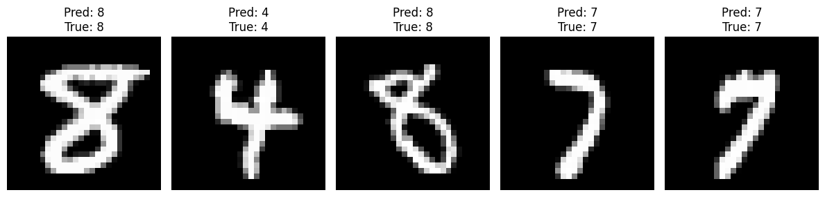
Making Predictions
Let's make predictions for the first 5 test samples:
predictions = model.predict(X_test[:5])
print("Predictions for the first 5 test samples:")
print(np.argmax(predictions, axis=1))
print("Actual labels:")
print(np.argmax(y_test[:5], axis=1))

# Visualize the predictions
plt.figure(figsize=(12, 4))
for i in range(5):
    plt.subplot(1, 5, i+1)
    plt.imshow(X_test[i].reshape(28, 28), cmap='gray')
    plt.title(f"Pred: {np.argmax(predictions[i])}\nTrue: {np.argmax(y_test[i])}")
    plt.axis('off')
plt.tight_layout()
plt.show()
Output:
Predictions for the first 5 test samples:
[8 4 8 7 7]
Actual labels:
[8 4 8 7 7]
Saving and Loading the Model
MicroKeras allows you to save and load models:
# Save the model
model.save('mnist_model.json')

# Load the model
loaded_model = Sequential.load('mnist_model.json')

# Compile the loaded model
loaded_model.compile(optimizer=optimizer,
                     loss='categorical_crossentropy',
                     metrics=['accuracy'])

# Evaluate the loaded model
loaded_test_loss, loaded_test_accuracy = loaded_model.evaluate(X_test, y_test)
print(f"Loaded model test accuracy: {loaded_test_accuracy:.4f}")
Output:
Loaded model test accuracy: 0.9671
Viewing Training History
Finally, let's print out the training history:
print("\nTraining History:")
print("Epoch\tAccuracy\tLoss")
for epoch, (accuracy, loss) in enumerate(zip(history['accuracy'], history['loss']), 1):
    print(f"{epoch}\t{accuracy:.4f}\t{loss:.4f}")
Output:
Training History:
Epoch	Accuracy	Loss
1	0.9235	14096.9166
2	0.9467	9728.8764
3	0.9592	7629.1049
4	0.9683	6160.9156
5	0.9730	5208.7316
6	0.9761	4604.9854
7	0.9803	3969.1862
8	0.9828	3443.3674
9	0.9831	3310.2258
10	0.9851	3007.7300
Running Tests
To ensure the library is functioning correctly, you can run the included tests:
- Run all tests:
pytest -v -s tests
- Run a specific test:
pytest -v -s tests/test_sigmoid.py
License
This project is licensed under the MIT License - see the LICENSE file for details.
1 maintainer

Metadata
1 maintainer
Release files for microkeras 0.1.4
For a detailed explanation of source distributions (sdists) and built distributions (wheels), please see the package formats documentation.
Source distribution (sdist)
| File | Size | Uploaded | |
|---|---|---|---|
| microkeras-0.1.4.tar.gz | 18.1 MB | Details |
Built distribution (wheel)
| File | Interpreter | ABI | Platform | Reset |
|---|---|---|---|---|
| microkeras-0.1.4-py3-none-any.whl | Python 3 | none | any | Details |
Total release size: 36.3 MB
Release files / microkeras-0.1.4.tar.gz
| Download URL | microkeras-0.1.4.tar.gz |
|---|---|
| Size | 18.1 MB |
| Tags | Source |
|
SHA-256 checksum How to use checksums |
3e775aa6e1d07efb41b0a62a7fff4725a7c828789943362c978a21531d3e87be
|
|
BLAKE2b-256 checksum How to use checksums |
843213bc81c59c0a1c048a4c38a560b07514ef6c641923a3c6f5e69ae8ce5a77
|
| Upload date | |
|
Uploaded using Trusted Publishing? What is trusted publishing? |
No |
| Uploaded via |
twine/5.1.0 CPython/3.12.7
|
Release files / microkeras-0.1.4-py3-none-any.whl
| Download URL | microkeras-0.1.4-py3-none-any.whl |
|---|---|
| Size | 18.2 MB |
| Tags | Python 3 |
|
SHA-256 checksum How to use checksums |
5dca1f4abe1b6f0e22601d0940731a777900442ee0b3994ccb98262db45f348c
|
|
BLAKE2b-256 checksum How to use checksums |
c083c66707059befac2c0870ccace243c3f60a27c3f9eb0abd5b6027257ca122
|
| Upload date | |
|
Uploaded using Trusted Publishing? What is trusted publishing? |
No |
| Uploaded via |
twine/5.1.0 CPython/3.12.7
|














