
minilink
Write the equations once. Simulate, analyze, control, plan, optimize, learn.





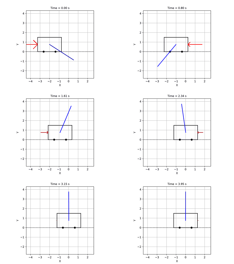
|
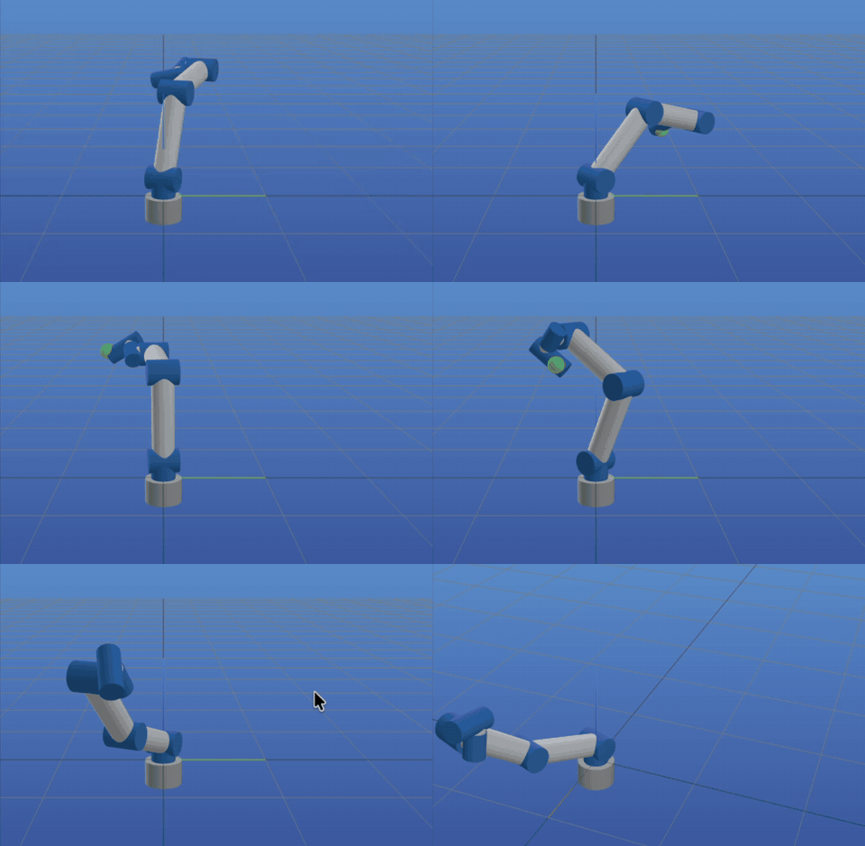
|
| trajectory optimization | task-space impedance control |
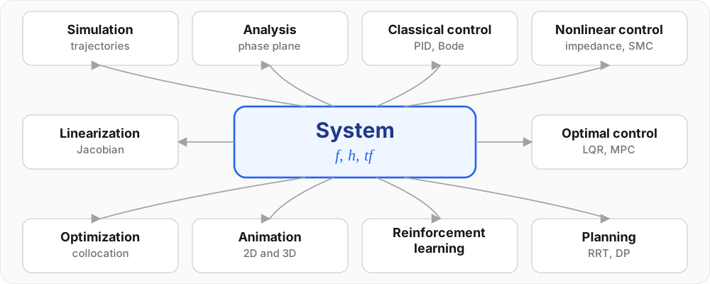
Minilink is an open-source Python toolbox for dynamical systems and control.
A model is a short class whose equations read like the textbook, and diagrams
are built from models with +, >> and @. Because every model, controller
and diagram is the same kind of object, one set of tools applies to all of
them: simulation and animation in 2D and 3D, frequency-domain analysis,
classical and state-space control, value iteration, sampling-based planning, trajectory
optimization, model predictive control and reinforcement learning. The same
equations compile and differentiate under JAX, so a course model is also a
research model.
Ten lines
from minilink import ImpedanceController, Pendulum

controller = ImpedanceController()
plant = Pendulum()

plant.x0[0] = 2.0
plant.params["l"] = 5.0
plant.params["m"] = 1.0

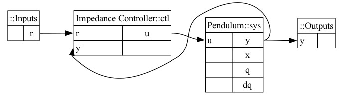
diagram = controller @ plant
diagram.compute_trajectory(tf=10.0)
diagram.plot_diagram()
diagram.plot_trajectory()
diagram.animate()
What is a System
A model is dynamics f, outputs h and body poses tf, functions of the
state x, the input u, the time t and the parameters params:
dx/dt = f(x, u, t; params)      dynamics
y     = h(x, u, t; params)      one per output port, default y = x
T     = tf(x, u, t; params)     body poses, for animation
Write f, and the plant simulates and plots. Add tf and a skin, and it
animates on matplotlib, plotly, meshcat (3D) or pygame, and you can drive it
from the keyboard:
import numpy as np
from minilink import DynamicSystem, Step
from minilink.core.kinematics import translation
from minilink.graphical.animation.primitives import Box, ground_line


class MassSpringDamper(DynamicSystem):
    # m p'' + c p' + k p = u

    def __init__(self):
        super().__init__(n=2, input_dim=1, output_dim=2)
        self.params = {"m": 1.0, "k": 4.0, "c": 0.3}
        self.skin = lambda sys: {
            "world": [ground_line(length=8.0)],
            "body": [Box(length_x=0.6, length_y=0.6, length_z=0.1)],
        }
        self.camera_scale = 4.0

    def f(self, x, u, t=0, params=None):
        p = self.params if params is None else params
        pos, vel = x
        acc = (u[0] - p["c"] * vel - p["k"] * pos) / p["m"]
        return np.array([vel, acc])

    def tf(self, x, u, t=0, params=None):
        return {"body": translation(x[0], 0.0, 0.0)}


msd = MassSpringDamper()
msd.x0[0] = 1.0
loop = Step(final_value=np.array([10.0]), step_time=2.0) >> msd
loop.compute_trajectory(tf=20.0)
loop.animate()  # renderer="plotly" | "meshcat" | "pygame"
# msd.game()    # keyboard drives u, live
f, h and tf are functions of (x, u, t; params) only: no hidden state on
the object. That one convention is what lets a model compose into diagrams,
run in batches and differentiate later. A diagram flattens to one state vector
and one f, so a closed loop linearizes, animates and nests like a plant.
One model, every tool
| Verb | Call |
|---|---|
| Simulate | plant.compute_trajectory(tf=10.0) |
| Frequency domain | plot_bode(plant, x_bar), plot_root_locus(C >> G) |
| Classical loop | PID(Kp, Ki, Kd) @ plant |
| State feedback | lqr_at_operating_point(plant, x_bar, Q, R) @ plant |
| Robot control | ComputedTorqueController(arm), JointImpedance(arm) |
| 3D robots | UR5Manipulator(), then animate(renderer="meshcat", is_3d=True) |
| Value iteration | DynamicProgrammingPlanner(problem, x_grid=(101, 101)) |
| Sampling search | RRTPlanner(problem) |
| Trajectory optimization | TrajectoryOptimizationPlanner(problem, transcription="direct_collocation") |
| Model predictive control | ModelPredictiveController(planner, dt_mpc=0.1) @ plant |
| Reinforcement learning | ReinforcementLearningPlanner(problem) |
| Sensitivity | plant.jacobian("f", "params", x_bar) |
The objects between the tools are the textbook's nouns. A PlanningProblem
is a system, a cost and boundary sets; every planner takes it and returns a
PlanningSolution (a policy, plus the trajectory when the solver computes one):
from minilink import (
    BallSet, DynamicProgrammingPlanner, Pendulum, PlanningProblem,
    QuadraticCost, RRTPlanner, TrajectoryOptimizationPlanner,
)

plant = Pendulum()
x_down, x_up = np.array([0.0, 0.0]), np.array([np.pi, 0.0])
problem = PlanningProblem(
    sys=plant, x_start=x_down, x_goal=x_up, Xf=BallSet(x_up, 0.2), tf=4.0,
    cost=QuadraticCost.from_system(plant, Q=np.eye(2), R=np.eye(1), xbar=x_up),
    X=plant.state.box,
)

vi = DynamicProgrammingPlanner(problem, x_grid=(101, 101), u_grid=(11,), dt=0.05)
vi.solve()                                   # value iteration on a grid
loop = vi.get_controller() @ plant           # the policy is a controller

rrt = RRTPlanner(problem, seed=0)
tree_traj = rrt.solve().trajectory           # kinodynamic tree search, bang-bang inputs

opt = TrajectoryOptimizationPlanner(problem, n_steps=40, transcription="direct_collocation")
opt_traj = opt.solve().trajectory            # direct collocation
Trajectory optimization transcribes the problem into a MathematicalProgram
solved by an Optimizer; a sampled controller closes the loop on the
continuous plant with ctl % dt, zero-order hold included.
Differentiable and compiled
The same f traces under JAX. One evaluator gives exact derivatives, batched
rollouts and gradients through a whole simulation:
ev = plant.compile(backend="jax")

A = plant.jacobian("f", "x", x_bar)               # exact linearization
S = plant.jacobian("f", "params", x_bar)          # sensitivity to each physical parameter
xs = ev.rollout_batch(x0s, n_steps=1000, dt=0.005,
                      params=dict(plant.params, l=lengths))   # a family of rod lengths, one call
Measured in the showcase notebook: 1000 rollouts of 1000 RK4 steps take
27 ms as a compiled batch and about 32 s one step at a time in Python
(Apple M4 Max). Derivatives are exact to machine precision, float64 by
default. Under the hood, compile() lowers a leaf or a wired diagram to flat
NumPy or JAX primitives (f, rk4_step, rk4_integrate_zoh,
rollout_batch); the trace tier (f_trace, f_trace_p) is what you
differentiate inside your own jit. See
07_compile and the
JAX showcase.
Two audiences, one codebase
- Teaching. NumPy, SciPy and Matplotlib are enough for simulation, phase
planes, animation, linearization, LQR and value iteration. Runs in Colab
from one setup cell. One import line covers a course:
from minilink import Pendulum, PID, lqr, PlanningProblem, ReinforcementLearningPlanner. - Research. Optional JAX for compile and autodiff, Ipopt for large NLPs,
meshcat for 3D, a hybrid stack for sampled MPC, a Gymnasium bridge
(
Sys2Gym) for external RL agents. Every catalog plant compiles on both backends.
The boundary between the two is a contract, not a convention: ROADMAP.md §2.
Install
Python 3.10+. Recommended: the conda environment from
environment.yml.
git clone https://github.com/alx87grd/minilink.git && cd minilink
conda env create -f environment.yml && conda activate minilink
conda env config vars set PYTHONPATH="$PWD" && conda deactivate && conda activate minilink
Or open any notebook in Colab: the first cell clones the repository. Basic tier, pip, and options: install.md.
Learn more
- Showcase notebook, the tool ladder on real plants
- JAX showcase, write
fonce, get every gradient - From RL to Bode showcase, six-axis robot, impedance loop, neural policy, frequency response and Lyapunov certificates
- Tutorial series 00–11, one notebook per package (core dynamics to reinforcement learning)
- Teaching notebooks, swing-up, DP, PPO, robot equations of motion
- Examples index, demos and projects by chapter
- API reference, DESIGN.md, ROADMAP.md, tests
- CONSTITUTION.md and RULES.md, the design law and the code rules every contributor and agent follows
Minilink is the successor of pyro, the toolbox behind the robotics and control courses at Université de Sherbrooke. MIT license.
1 maintainer

Download files
Download the file for your platform. If you're not sure which to choose, learn more about installing packages.
Source Distribution
Built Distribution
Filter files by name, interpreter, ABI, and platform.
If you're not sure about the file name format, learn more about wheel file names.
Copy a direct link to the current filters
File details
Details for the file minilink-0.1.0.tar.gz.
File metadata
- Download URL: minilink-0.1.0.tar.gz
- Upload date:
- Size: 3.1 MB
- Tags: Source
- Uploaded using Trusted Publishing? Yes
- Uploaded via:
twine/7.0.0 CPython/3.13.14
File hashes
| Algorithm | Hash digest | |
|---|---|---|
| SHA256 |
6a60d0f8bb5c08e954377f92e89ed89813feca6e38ec0c2d3328788e9d6b2505
|
|
| MD5 |
39db402e3e1672eacc36e48e1957ea92
|
|
| BLAKE2b-256 |
736212905d02de78dd4b0844a9fbcdbc260289330af470a536ddcdbd5a66f495
|
Provenance
The following attestation bundles were made for minilink-0.1.0.tar.gz:
Publisher:
publish.yml on alx87grd/minilink
-
Statement:
-
Statement type:
https://in-toto.io/Statement/v1 -
Predicate type:
https://docs.pypi.org/attestations/publish/v1 -
Subject name:
minilink-0.1.0.tar.gz -
Subject digest:
6a60d0f8bb5c08e954377f92e89ed89813feca6e38ec0c2d3328788e9d6b2505 - Sigstore transparency entry: 2866358812
- Sigstore integration time:
-
Permalink:
alx87grd/minilink@47cfd50e4f6c2a0d25c07ec3a1ae40a97a82ecec -
Branch / Tag:
refs/tags/0.1.0 - Owner: https://github.com/alx87grd
-
Access:
public
-
Token Issuer:
https://token.actions.githubusercontent.com -
Runner Environment:
github-hosted -
Publication workflow:
publish.yml@47cfd50e4f6c2a0d25c07ec3a1ae40a97a82ecec -
Trigger Event:
push
-
Statement type:
File details
Details for the file minilink-0.1.0-py3-none-any.whl.
File metadata
- Download URL: minilink-0.1.0-py3-none-any.whl
- Upload date:
- Size: 553.6 kB
- Tags: Python 3
- Uploaded using Trusted Publishing? Yes
- Uploaded via:
twine/7.0.0 CPython/3.13.14
File hashes
| Algorithm | Hash digest | |
|---|---|---|
| SHA256 |
84ad4bed69189d7417d4fedf9d4364a40a82dee8511d093b104ddac5f37e3aa9
|
|
| MD5 |
d5e307320b3ae8358a7be01b48604a79
|
|
| BLAKE2b-256 |
3b9729f3be6352bbad791652718a17ff81181b6dd6236c2fe88e45a777706e1d
|
Provenance
The following attestation bundles were made for minilink-0.1.0-py3-none-any.whl:
Publisher:
publish.yml on alx87grd/minilink
-
Statement:
-
Statement type:
https://in-toto.io/Statement/v1 -
Predicate type:
https://docs.pypi.org/attestations/publish/v1 -
Subject name:
minilink-0.1.0-py3-none-any.whl -
Subject digest:
84ad4bed69189d7417d4fedf9d4364a40a82dee8511d093b104ddac5f37e3aa9 - Sigstore transparency entry: 2866358859
- Sigstore integration time:
-
Permalink:
alx87grd/minilink@47cfd50e4f6c2a0d25c07ec3a1ae40a97a82ecec -
Branch / Tag:
refs/tags/0.1.0 - Owner: https://github.com/alx87grd
-
Access:
public
-
Token Issuer:
https://token.actions.githubusercontent.com -
Runner Environment:
github-hosted -
Publication workflow:
publish.yml@47cfd50e4f6c2a0d25c07ec3a1ae40a97a82ecec -
Trigger Event:
push
-
Statement type:













