
Mirabolic
Tools for statistical modeling and analysis, written by Mirabolic. These modules can be installed by running
pip install --upgrade mirabolic
and the source code can be found at https://github.com/Mirabolic/mirabolic
Table of Contents
- Visualizing LLM Embeddings
- Comparing Event Rates
- CDFs With Confidence Intervals
- Neural Nets for GLM regression
Visualizing LLM Embeddings
Suppose we have a collection of paragraphs describing different things. We can use an LLM to "embed" those paragraphs, i.e., convert them into vectors in some high dimensional space. (In concrete terms: each paragraph is converted into a list of about 3000 numbers). Because of the magic of LLMs, similar paragraphs are supposed to cluster near each other in this high-dimensional space.
But how do we know if that's actually happening? Well, we might be lucky enough to have labels describing a few types paragraphs. If that's the case, we can map the embeddings down to two dimensions, color the points by label, and look at the scatter plot. If our embeddings are working correctly, points with the same color will group together.
Installation
Because this code invokes LLMs, we require a little extra setup. In particular, we use OpenAI's embedding models, which means that you, dear reader, need an OpenAI API key. For those unfamiliar with this process, we offer a primer.
To get an OpenAI API key
1 Get a developer account on OpenAI. (You'll need a credit card, I'm afraid. FWIW, small experiments typically cost several cents.)
2 Get an API key. This is a string of letters and numbers that begins sk-.
Now that you have the API key, you need to store it where your system can find it. This can be writing a file called .env and sticking in the API key. (If you already have a file like that, just add this as an extra line). The contents of your file should look like this:
OPENAI_API_KEY=sk-...
When you run this code, it will look for a .env file in the current directory; if it doesn't find it, it will look in the parent directory, and the parent's parent directory, and so on. This means that if you'd like, you can put the .env file in your home directory and code you execute will find it. If you're not running in a home directory, just make sure that there is a .env file in whatever directory you use.
A word of warning: this key should stay secret. If you're working in a Git repo, be sure to .gitignore the .env file so you do not accidentally commit it.
Examples
We provide an example, but first, let's make some data. (Note that here our "paragraph" is only one or two words.)
# Make some data that falls into natural classes
dog_breeds = ["Labrador Retriever", "German Shepherd", "Golden Retriever", "Bulldog", "Poodle", "Beagle", "Rottweiler", "Yorkshire Terrier", "Boxer", "Dachshund"]
cat_breeds = ["Siamese", "Persian", "Maine Coon", "Ragdoll", "Bengal", "Sphynx", "British Shorthair", "Abyssinian", "Scottish Fold", "Russian Blue"]
common_birds = ["Northern Cardinal", "American Robin", "Blue Jay", "House Sparrow", "Mourning Dove", "European Starling", "Black-capped Chickadee", "American Goldfinch", "Red-winged Blackbird", "Downy Woodpecker"]

data = dog_breeds + cat_breeds + common_birds
labels = len(dog_breeds) * ["dog"] + len(cat_breeds) * ["cat"] + len(common_birds) * ["birds"]
Next, let's use an LLM to embed the data in a high dimension, then visualize it in two dimensions:
import mirabolic

embedder = mirabolic.llm_embedder(X=data, L=labels)
embedder.run_all()
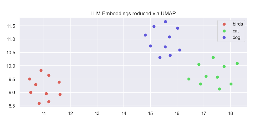
Wow! Nice grouping of categories.
Sometimes we might want to process the text before embedding it. The llm_embedder() allows for arbitrary text transformations. Here's an example in which the transformation itself invokes another LLM.
import mirabolic

def f(s):
    """
    Replace the breed or species with a pet name.
    """
    prompt = (
        f"I have a pet {s}. I need a name for my pet that is "
        "some sort of outrageous pun that will reveal its breed or species. "
        "Please reply with one name (and no other text)."
    )
    response = mirabolic.LLM_API(prompt)
    print(f"{s}  =>  {response}")
    return response

embedder = mirabolic.llm_embedder(X=data, L=labels, f=f)
embedder.run_all()
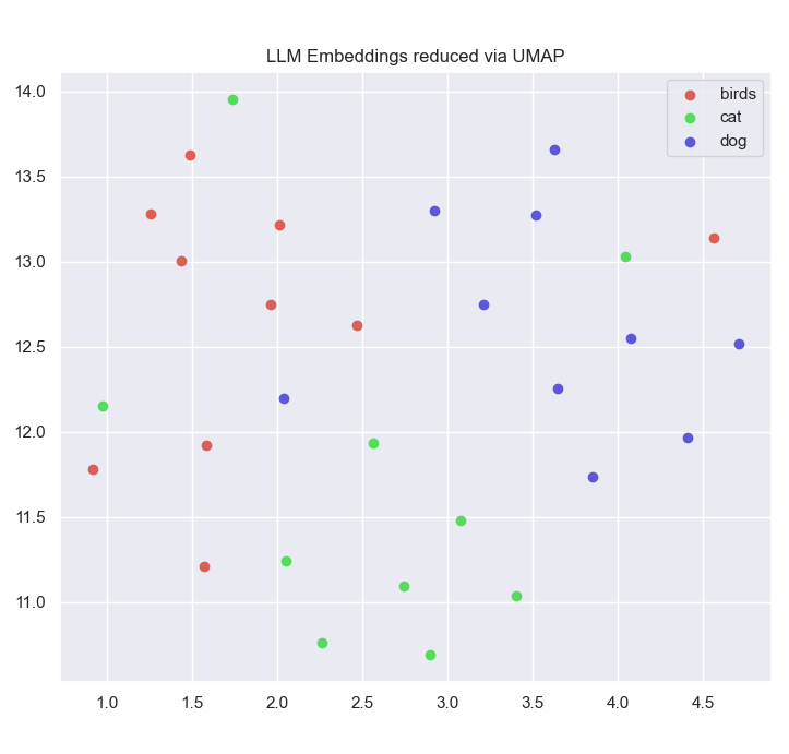
So, we transform the species name into a cutesy pet name (e.g., Boxer -> Rocky Bal-bow-wow, or Russian Blue -> Czar Purrtin). Of course, this makes it more difficult to distinguish the underlying species, so the clusters become murkier. Nevertheless, the cat/dog/bird regions are still fairly visible:
Comparing Event Rates
Suppose you run a website. Every day you run a new email campaign to drive traffic to your site. You're considering a new approach, so you A/B test your campaigns: a portion of your emails use the new style of campaign and the rest use the old style.
Which style won? The new campaign looks good, but how do you know it's not just a random fluke? You vaguely remember an old stats teacher saying something about designing experiments with sufficient statistical power for a target effect size, but you don't know what the effect size is going to be, and you've already run the experiment! You really just want some simple way of visualizing the data you already have to see if the new style of campaigns are an improvement, or if it's all just random noise.
We provide such a tool here:
import numpy as np
import mirabolic
import matplotlib.pyplot as plt

# Make some synthetic data
num_campaigns = 8
num_emails = 3000  # Number of emails in one arm of one campaign
# In this example, the "B" arm has a slightly higher conversion rate
num_conversions_A = np.random.binomial(num_emails, 0.03, size=num_campaigns)
num_conversions_B = np.random.binomial(num_emails, 0.04, size=num_campaigns)
num_emails_A = num_campaigns * [num_emails]
num_emails_B = num_campaigns * [num_emails]

# Plot the figure
plt.figure(figsize=(6, 6))
results = mirabolic.rate_comparison(
    num_successes_A=num_conversions_A,
    num_successes_B=num_conversions_B,
    num_trials_A=num_emails_A,
    num_trials_B=num_emails_B,
)
plt.show()
Here's the output:
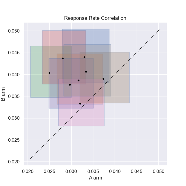
The figure shows a scatter plot with 8 points. Each point corresponds to a campaign, where the x-value is the conversion rate for the A arm (the old style, say) and the y-value is the conversion rate for the B arm (the new style). Around each point is a confidence rectangle showing how seriously to take it. If all the rectangles overlap with the diagonal line, then you don't have enough data to draw any conclusions (at least from individual campaigns). If the rectangles mostly fall above the dotted line, then the new style is an improvement; if below, it's making things worse.
CDFs with Confidence Intervals
When exploring data, it can be very helpful to plot observations as a cumulative density function, or CDF. (In medical contexts, doctors study the "survival function", which is 1 minus the CDF and essentially amounts to the same thing.) We plot a CDF by sorting the observed data from smallest to largest value. We can treat1 the value in the middle of the sorted list as approximately the median, the value 90% of the way up the list as near the 90th percentile, and so forth.
When interpreting a CDF, or comparing two of them, one often wishes for something akin to a confidence interval. How close is the middle value to the median? Somewhat surprisingly, it is possible to compute the corresponding confidence intervals exactly.2
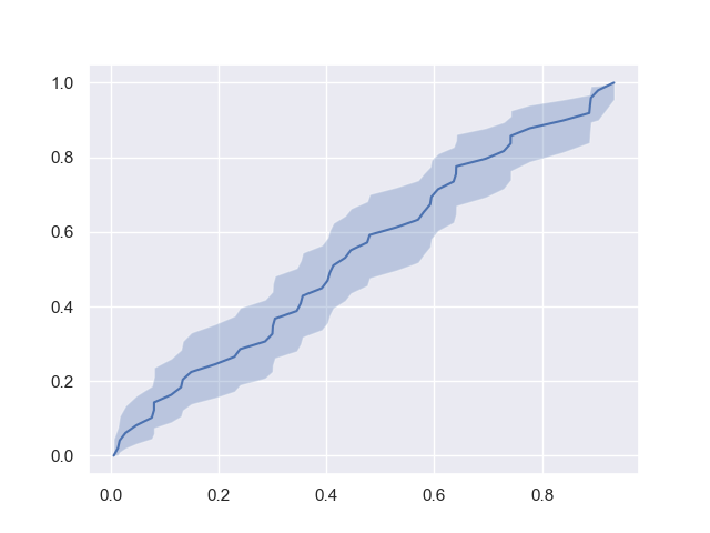
For a single data point, the uncertainty around its quantile can be thought of as a confidence interval. If we consider all the data points, then we refer to a confidence band.3
We provide a simple function for plotting CDFs with confidence bands; one invokes it by calling something like:
import mirabolic
import matplotlib.pyplot as plt
import random

data = [random.random() for _ in range(50)]
mirabolic.cdf_plot(data=data)
plt.show()
The figure looks like this:
More examples can be found in mirabolic/cdf/sample_usage.py.
Neural Nets for GLM regression
GLMs (Generalized Linear Models) are a relatively broad class of statistical model first popularlized in the 1970s. These have grown popular in the actuarial literature as a method of predicting insurance claims costs and frequency.
With the appropriate loss function, GLMs can be expressed as neural nets. These two techniques have traditionally been treated as distinct, but bridging the divide provides two advantages.
First, a vast amount of effort has been spent on optimizing and accelerating neural nets over the past several years (GPUs and TPUs, parallelization). By expressing a GLM as a neural net, we can leverage this work.4
Second, expressing a GLM as a neural net opens the possibility of extending the neural net before or after the GLM component. For instance, suppose we build three subnets that each computed a single feature, and then feed the three outputs as inputs into the Poisson regression net. This single larger network would allow the three subnets to engineer their individual features such that the loss function of the joint network was optimized. This approach provides a straightforward way of performing non-linear feature engineering but retaining the explainability of a GLM. This two-step approach may provide regulatory advantages, since US Departments of Insurance (DOIs) have been reluctant to approve end-to-end deep learning models.
We provide loss functions for several of the most commonly used GLMs. Minimal code might look something like this:
import mirabolic.neural_glm as neural_glm
from keras.models import Sequential
import tf

model = Sequential()
# Actually design your neural net...
# model.add(...)
loss=neural_glm.Poisson_link_with_exposure
optimizer = tf.keras.optimizers.Adam()
model.compile(loss=neural_glm, optimizer=optimizer)
To illustrate this process in more detail, we provide code to perform Poisson regression and Negative Binomial regression using a neural net.
To see the code in action, grab the source code from GitHub, then change to this directory, and run
python run_examples.py
This will generate Poisson-distributed data and corresponding features and then try to recover the "betas" (i.e., the linear coefficients of the GLM) using various models, outputting both the true and recovered values.
-
We assume the data consists of i.i.d. draws from some unknown probability distribution. ↩
-
More precisely, suppose we draw a sample of n i.i.d. observations and consider the i-th smallest; if we are sampling from any continuous probability distribution, then the distribution of the corresponding quantile has a Beta distribution, B(i, n-i+1). ↩
-
Because we have access to a prior distribution on quantiles, these are arguably credible intervals and credible bands, rather than confidence intervals and bands. We do not concern ourselves with this detail. ↩
-
In terms of focus, this chart suggests something of the explosion of interest in neural nets and deep learning relative to more traditional actuarial models. ↩
1 maintainer

Download files
Download the file for your platform. If you're not sure which to choose, learn more about installing packages.
Source Distribution
Built Distribution
Filter files by name, interpreter, ABI, and platform.
If you're not sure about the file name format, learn more about wheel file names.
Copy a direct link to the current filters
File details
Details for the file mirabolic-0.3.10.tar.gz.
File metadata
- Download URL: mirabolic-0.3.10.tar.gz
- Upload date:
- Size: 35.9 kB
- Tags: Source
- Uploaded using Trusted Publishing? No
- Uploaded via:
twine/5.1.0 CPython/3.12.5
File hashes
| Algorithm | Hash digest | |
|---|---|---|
| SHA256 |
355f1a149bcd48322327aa8568a9a6c7c415d9d3086d7c797070d333e2970587
|
|
| MD5 |
2714991da2f0193328c2bfec29a9125d
|
|
| BLAKE2b-256 |
87a41cd4895bfc5d8f9e9644b7c1d017f2d56f213f9fe794317787da022b2e0b
|
File details
Details for the file mirabolic-0.3.10-py3-none-any.whl.
File metadata
- Download URL: mirabolic-0.3.10-py3-none-any.whl
- Upload date:
- Size: 34.7 kB
- Tags: Python 3
- Uploaded using Trusted Publishing? No
- Uploaded via:
twine/5.1.0 CPython/3.12.5
File hashes
| Algorithm | Hash digest | |
|---|---|---|
| SHA256 |
7fb0da0fbaf9a8309b451f4b9013202461ede020578371fa172ee3934468e322
|
|
| MD5 |
07763e2c5ff2a8977446d4f4423f6b9b
|
|
| BLAKE2b-256 |
2dc4fd6f6e1ffb183f3ab7a245086cd3403d5113a5cf69e56fc9b2f64bc05742
|














