
mllpanel




Machine learning based panel data models with fixed effects and cross-sectional dependence.
A complete, tested Python implementation of
Yang, B., Long, W. and Cai, Z. (2024). Machine Learning Based Panel Data Models. Working paper.
mllpanel estimates a panel regression in which the functional form is
unknown, the individual effects may be correlated with the regressors, and
the errors carry an unobserved factor structure — using any machine learning
method for the unknown function, and no proxy variable and no instrument for
the latent terms.
📖 Start here: the researcher's guide
→ docs/GUIDE.md — How to write a complete application
An 18-section walkthrough from a raw panel to manuscript-ready tables and figures: is the method right for your data, how to diagnose whether you actually have these problems, how to choose a learner and a specification, how to check condition (C3) before believing anything, which standard errors to report, how to read a nonparametric production function, how to benchmark against Olley–Pakes and Levinsohn–Petrin, how to forecast — plus the complete script, a 12-row pitfalls table and a reporting checklist for referees.
Supporting documents:
| Document | What it covers |
|---|---|
| GUIDE.md | The researcher's guide — read this first |
| SYNTAX.md | Complete argument-by-argument reference for every class and function |
| THEORY.md | The derivation equation by equation, a fidelity map from paper equations to code, every deviation with its justification, and an errata list for the published paper |
| CHANGELOG.md | Release notes |
| examples/ | Six runnable scripts |
Contents
- The problem this solves
- The method
- Install
- Sixty seconds
- API tour
- Real economic data, bundled
- Two results the paper does not report
- Reproducing the paper
- Specifications
- Learners
- Standard errors
- Faithfulness to the paper
- Tables and figures
- Cost and performance
- Troubleshooting
- Testing
- Citation
- License
The problem this solves
Suppose you want to estimate a production function, a demand curve, or an asset pricing relation on panel data, and three things are true at once:
- You do not want to impose a functional form. Cobb–Douglas is a restriction, not a finding.
- Unit-level heterogeneity is correlated with your regressors. Firms with high unobserved productivity hire more labour, so OLS is biased.
- There are shocks that hit everyone at once. A business cycle, an oil price shock, a policy change. These make the errors cross-sectionally dependent and — if they also move your regressors — endogenous.
The standard toolkit forces a choice. Nonparametric panel estimators (sieves, kernels) handle (1) but collapse under the curse of dimensionality beyond one or two regressors. Machine learning panel methods handle (1) and scale, but existing ones either pool the data outright or put fixed effects in as predictors, leaving (3) untouched. Control-function estimators (Olley–Pakes, Levinsohn–Petrin) handle (2) but require a proxy variable, impose a parametric production function, and say nothing about (3).
This method handles all three simultaneously, and needs no proxy. The insight — from Mundlak (1978), Pesaran (2006) and Huang (2013) — is that both latent terms are spanned by observable averages, so they can be replaced by regressors you can compute. What is left is a partially linear model, which the debiased machine learning of Chernozhukov et al. (2018) estimates with any learner you like.
When not to use it: if you are happy with a linear form, a two-way fixed
effects regression is faster and has cleaner inference. If your application
turns on heterogeneity in the factor loadings, this method implicitly assumes
that away — see
THEORY.md §2.
And it needs both N and T reasonably large; see the sample-size table in
GUIDE.md §1.
The method
The model — the paper's equation (1):
$$ y_{it} = f(x_{it}) + \alpha_i + \gamma_i'\lambda_t + \varepsilon_{it} $$
with $f$ unknown, the fixed effects $\alpha_i$ freely correlated with $x_{it}$, and the common factors $\lambda_t$ also allowed to correlate with $x_{it}$.
The trick — the paper's equation (2), derived in its Appendix A by a Taylor expansion inside a shrinking neighbourhood of $x$. Both latent terms are spanned by observable averages: the fixed effects by time averages, the common factors by cross-sectional averages. So the model becomes partially linear:
$$
y_{it} = f(x_{it}) + \beta' z_{it} + e_{it},
\qquad
z_{it} = \bigl(\underbrace{\bar y_t - \bar y,\ (\bar x_t - \bar x)'}{\text{spans } \lambda_t},
\underbrace{\bar y_i - \bar y,\ (\bar x_i - \bar x)'}{\text{spans } \alpha_i}\bigr)'
$$
The estimation — equations (3)–(6):
- Partial out $g = E(y\mid x)$ and $m = E(z\mid x)$ by machine learning.
- Cross-fit over the time index. Folds are over periods, not observations: every unit in period $t$ shares a fold, which is what stops $\lambda_t$ leaking across the split.
- Solve the Neyman-orthogonal moment condition in closed form.
- Recover $f$ from a second-stage regression of $y - \hat\beta'z$ on $x$.
Why the orthogonality matters: it makes $\hat\beta$ robust to first-order error in the nuisance estimates. That is what lets you use a random forest for $f$ without regularisation bias contaminating everything else.
Install
From PyPI:
pip install mllpanel
With figures and parallel Monte Carlo:
pip install "mllpanel[plots,parallel]"
From source, for development:
git clone https://github.com/merwanroudane/mllpanel.git
cd mllpanel
pip install -e ".[dev]"
pytest -q
| Extra | Adds | For |
|---|---|---|
| (none) | numpy, pandas, scikit-learn, scipy |
estimation, tables |
plots |
matplotlib |
all figures |
parallel |
joblib |
n_jobs= in Monte Carlo and cross-fitting |
dev |
the above + pytest, tabulate, openpyxl |
tests, Markdown tables, xlsx export |
Requires Python ≥ 3.9. The four real datasets ship inside the wheel, so every example in this documentation runs offline.
Sixty seconds
from mllpanel import MLLPanel
from mllpanel.datasets import load_snmesp

df = load_snmesp()          # 738 Spanish manufacturing firms x 8 years, real data

model = MLLPanel(
    learner="rf",           # random forest for the unknown production function
    spec="crfe",            # cross-sectional AND time averages
    vcov="twoway",          # two-way clustered standard errors
    random_state=0,
).fit(df, y="y", x=["n", "k"], unit="firm", time="year")

print(model.summary())
====================================================================================
                      Machine Learning Based Panel Data Model
               Yang, Long and Cai (2024) - debiased machine learning
====================================================================================
Dep. variable     y                       No. observations                    5904
Specification     CR + FE                 No. units (N)                        738
Learner (g, m, f) Random Forests          No. periods (T)                        8
Cross-fitting     K=5, block              Panel                           balanced
beta aggregation  pooled                  Covariates (d)                         2
                                          Augmented regressors                   6
Std. errors       Two-way clustered (unit and period)
------------------------------------------------------------------------------------
                    Parametric component of  y = f(x) + b'z + e
------------------------------------------------------------------------------------
Regressor                    Coef.   Std. err.           z       P>|z|  [2.5%  97.5%]
  Cross-sectional averages (common factors)
ybar_t                      1.0020      0.0812     12.3390      0.0000  0.8429  1.1612
xbar_t[n]                  -0.4200      0.4323     -0.9716      0.3313 -1.2673  0.4273
xbar_t[k]                  -0.4202      0.1017     -4.1320      0.0000 -0.6195 -0.2209
  Time averages (fixed effects)
ybar_i                      0.9729      0.0046    210.1484      0.0000  0.9639  0.9820
xbar_i[n]                  -0.6753      0.0336    -20.1247      0.0000 -0.7411 -0.6096
xbar_i[k]                  -0.2874      0.0291     -9.8839      0.0000 -0.3444 -0.2304
------------------------------------------------------------------------------------
Specification tests
  H0: cross-sectional averages jointly zero (no unobserved common factors)
    chi2(3) = 566.9690    p = 0.0000
  H0: time averages jointly zero (individual effects uncorrelated with x; Mundlak)
    chi2(3) = 52015.0492    p = 0.0000
------------------------------------------------------------------------------------
Fit:  R2 = 0.9976   R2 (uncentred, GKX) = 0.9999   RMSE = 0.0677
Nuisance out-of-fold R2:  g = 0.8588   m: min -0.4677, median 0.2330, max 0.9900
====================================================================================
A free correctness check is built into that output. Appendix A of the paper
implies a coefficient of exactly one on both ybar_t and ybar_i when
loadings are homogeneous, and minus the input elasticity on xbar_i[·]. The
estimates are 1.002 and 0.973, with −0.675 and −0.287 against elasticities of
+0.63 and +0.33. If your own fit does not show this pattern, stop and
investigate before interpreting anything.
Then read the economics off the nonparametric part:
ape = model.partial_effects()          # output elasticities, since y and x are logs
print(ape[["APE", "Median"]].round(3))
#             APE  Median
# n         0.627   0.132
# k         0.334   0.226
print("Returns to scale:", round(ape["APE"].sum(), 3))   # 0.961

prod = model.productivity()            # firm-year TFP decomposition
API tour
Fifteen modules. Full signatures in SYNTAX.md.
The estimator
from mllpanel import MLLPanel, fit_mllpanel

MLLPanel(
    learner="lasso", spec="crfe", *,
    learner_f=None, learner_m=None,          # different learners per stage
    n_folds=5, fold_scheme="block",          # cross-fitting
    drop_remainder=False, beta_agg="pooled",
    vcov="twoway", vcov_lags=None,
    f_crossfit=False, grand_mean="obs",
    ybar_forecast_learner="ols",
    alpha=0.05, random_state=None,
    store_models=False, n_jobs=None, verbose=False,
)
Three interchangeable call styles:
model.fit(df, y="gsp", x=["emp", "pc"], unit="state", time="year")   # DataFrame
model.fit(panel_data_object)                                        # PanelData
model.fit(y=y_arr, x=X_arr, unit=id_arr, time=t_arr)                # arrays
Key fitted attributes:
| Attribute | Meaning |
|---|---|
beta_, vcov_, inference_ |
$\hat\beta$, its covariance, the full coefficient table |
wald_ |
block tests: "common_factors", "fixed_effects" |
f_, f_hat_ |
the fitted second-stage model, and $\hat f(x_{it})$ |
fittedvalues_, resid_ |
$\hat y$ and $y-\hat y$ |
nuisance_fit_ |
out-of-fold $R^2$ per nuisance regression — the practical check on condition (C3) |
z_, z_tilde_, y_tilde_ |
augmented regressors and their cross-fitted residualised versions |
r2_, r2_uncentered_, rmse_ |
centred $R^2$ (report this), the paper's uncentred one, RMSE |
folds_, used_, n_dropped_ |
the time-index partition and what entered the score |
Methods:
model.predict(df_new, unit="firm", time="year",
              ybar_t_source="auto",     # "model" for honest forecasting
              unseen_units="error",
              return_components=False)
model.predict_f(X)                      # f-hat alone; levels not identified
model.partial_effects(relative_step=0.05)     # elasticities, if y and x are logs
model.partial_dependence("k", n_grid=60, at="average")
model.productivity()                    # f_hat, factor_part, fe_part, tfp_hat
model.summary(); model.summary_frame(); model.info(); model.to_latex()
Diagnostics
from mllpanel.diagnostics import cd_test, dependence_report, residual_diagnostics

cd_test(model.resid_, unit, time)       # Pesaran CD + mean |rho|
dependence_report(df, y, x, unit, time, specs=("pooled","fe","cr","crfe"))
Simulation and Monte Carlo
from mllpanel import simulate_panel, time_split, run_design, run_sensitivity
from mllpanel.montecarlo import (paper_designs, inference_study,
                                 theoretical_beta, estimate_runtime, aggregate)

df = simulate_panel(n_units=10, n_times=100, d=5, c1=1.0, c2=1.0,
                    ftype="type1", gamma=0.5, factor_ar=0.0, seed=0)
parts = time_split(df, fractions=(0.3, 0.2, 0.5))       # consecutive periods

results = run_design(paper_designs(), learners=("lasso","rf","nn"),
                     n_reps=1000, n_jobs=8)
agg = aggregate(results)                 # + Monte Carlo standard errors
Production functions
from mllpanel.tfp import (estimate_pooled, estimate_fe, estimate_op,
                          estimate_lp, estimate_acf,
                          specification_table, comparison_table)

fits = [estimate_pooled(df, "y", ["n","k"], "firm", "year", cluster="firm"),
        estimate_fe(df, "y", ["n","k"], "firm", "year", effects="twoway"),
        estimate_op(df, "y", "n", "k", "log_inv", "firm", "year"),
        estimate_lp(df, "y", "n", "k", "i", "firm", "year"),
        estimate_acf(df, "y", "n", "k", "i", "firm", "year")]
specification_table(fits)                                       # Table 7
comparison_table(fits, df, {"ln M": "i", "ln I": "log_inv"})     # Table 8
Output
from mllpanel.tables import save_table, montecarlo_table, table_to_latex
from mllpanel.plots import (set_style, save_figure, plot_sensitivity,
                            plot_coefficients, plot_partial_dependence,
                            plot_surface, plot_factor_path, plot_tfp,
                            plot_nuisance_quality, plot_dependence_report)

set_style()                                        # 9 pt serif, journal defaults
save_table(tab, "out/table_1", formats=("csv","tex","md"),
           caption="...", label="tab:1", notes="...", highlight_min=True)
save_figure(plot_surface(model, "n", "k"), "out/fig_3", formats=("pdf","png"))
Meta
import mllpanel
mllpanel.__version__
print(mllpanel.deviations())          # every implementation choice, at runtime
print(mllpanel.citation("bibtex"))
Module map
| Module | Contents |
|---|---|
mllpanel.core |
MLLPanel — the estimator |
mllpanel.panel |
PanelData, the six averages, build_z |
mllpanel.crossfit |
sample splitting over the time index, three schemes |
mllpanel.learners |
LASSO, random forests, 32-16-8 network, plus five more |
mllpanel.tune |
validation-block hyper-parameter selection (the paper's protocol) |
mllpanel.inference |
five sandwich estimators, Wald tests on each block |
mllpanel.metrics |
$MSE(f)$, in- and out-of-sample $R^2$, centred and uncentred |
mllpanel.simulate |
the DGP of equation (7), Type 1 and Type 2, the 30/20/50 split |
mllpanel.montecarlo |
Tables 1–6, Figures 1–6, inference study, runtime estimation |
mllpanel.tfp |
pooled, two-way FE, Olley–Pakes, Levinsohn–Petrin, ACF, Tables 7–8 |
mllpanel.diagnostics |
Pesaran CD test, serial correlation, dependence_report |
mllpanel.tables |
booktabs LaTeX, Markdown, CSV, xlsx |
mllpanel.plots |
ten journal-quality figure types |
mllpanel.colors |
MATLAB parula, Okabe–Ito colour-blind-safe palette |
mllpanel.datasets |
four real economic panels |
Examples
| Script | What it does |
|---|---|
01_quickstart.py |
the minimum viable application |
02_real_data_tfp.py |
the full Section 4 exercise: 3 learners, 6 benchmarks, Tables 7–8, 8 figures. Copy this one. |
03_replicate_tables.py |
Monte Carlo Tables 1–6 |
04_replicate_figures.py |
Monte Carlo Figures 1–6 |
05_forecasting.py |
out-of-sample and rolling one-step-ahead forecasts |
06_inference_study.py |
coverage of the Theorem 1 sandwich |
Real economic data, bundled
The paper's own application uses licensed CSMAR data on Chinese A-share firms, which cannot be redistributed. Four public panels ship inside the wheel.
| Loader | $N$ | $T$ | Balanced | Why it is here |
|---|---|---|---|---|
load_snmesp() |
738 | 8 | yes | Spanish manufacturing, 1983–1990. Log output, labour, capital and log intermediate consumption, so it supports the full Table 8 comparison against OP, LP and ACF. The closest public analogue of the paper's Section 4, which used 459 Chinese firms over 20 years. |
load_produc() |
48 | 17 | yes | US states, 1970–1986. Real gross state product, labour, private and public capital. Small $N$, long $T$. |
load_grunfeld() |
10 | 20 | yes | Firm investment, 1935–1954. $N=10$ makes the $O(1/N)$ simultaneity of the CCE step visible. A cautionary example. |
load_empluk() |
140 | 7–9 | no | UK firms, 1976–1984. For checking that your code path handles unequal $T_i$. |
Sources: Alonso-Borrego and Arellano (1999); Munnell (1990); Grunfeld (1958);
Arellano and Bond (1991) — all redistributed from the R package plm (GPL-2).
snmesphas no investment series, solog_invis imputed from $I_{it}=K_{it}-(1-\delta)K_{i,t-1}$. This is non-positive for 15.5% of the panel — not a defect, but exactly the censoring the paper cites as the motivation for Levinsohn–Petrin over Olley–Pakes. Because it is imputed rather than measured, its column in a Table 8 replication is not numerically comparable to the paper's.
Two results the paper does not report
1. The cross-sectional averages really do absorb the dependence
The paper's central claim is directly testable, and the paper does not test it.
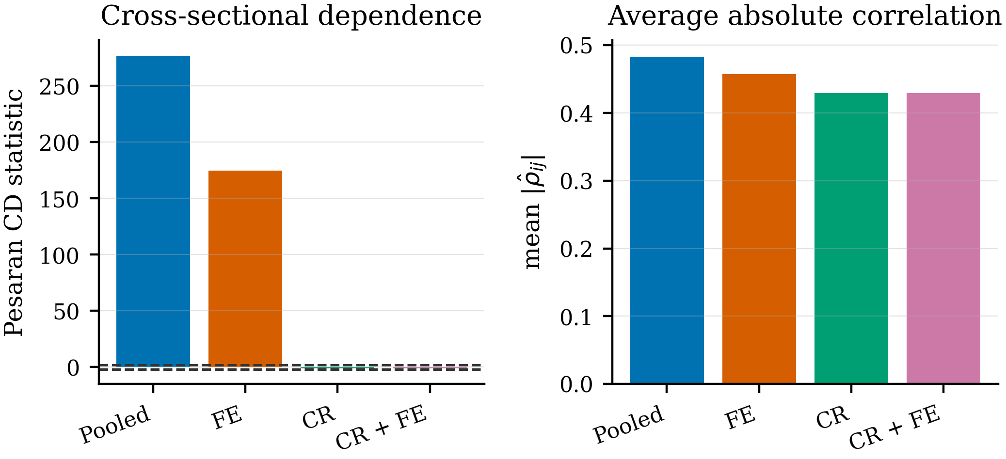
diagnostics.dependence_report does. On the Spanish panel:
| Specification | Pesaran CD | p-value | mean ρ | mean |ρ| |
|---|---|---|---|---|
| Pooled | 276.60 | 0.000 | 0.188 | 0.483 |
| FE | 174.80 | 0.000 | 0.119 | 0.457 |
| CR | −1.05 | 0.293 | −0.001 | 0.429 |
| CR + FE | −1.14 | 0.253 | −0.001 | 0.430 |
The CD statistic collapses from 277 to −1.1. Adding additive fixed effects barely helps (175) — a factor structure is not an additive effect, which is the paper's Panel C result appearing in real data.
But read the last column. Mean absolute pairwise correlation moves only
from 0.483 to 0.430. The CD test has no power against a factor structure whose
loadings average to zero, so together these columns say the block removes the
average co-movement while individual firm pairs remain strongly correlated.
mllpanel reports both, always.
2. Which standard errors actually work
Theorem 1 gives $\Sigma^{-1}V\Sigma^{-1}$ but supplies no sample analogue,
and the paper reports no standard errors anywhere and runs no coverage
experiment. examples/06_inference_study.py runs one — Type 1 design, $N=20$,
$T=200$, $d=5$, 150 replications, against the closed-form $\beta$ from
Appendix A:
vcov |
CR block se_ratio | CR coverage | FE block se_ratio | FE coverage |
|---|---|---|---|---|
theorem1 (i.i.d. plug-in) |
6.63 | 1.000 | 16.37 | 1.000 |
cluster_unit |
6.75 | 1.000 | 0.86 | 0.892 |
cluster_time |
0.92 | 0.912 | 16.87 | 1.000 |
dk (Driscoll–Kraay) |
0.92 | 0.908 | 16.66 | 1.000 |
twoway (default) |
3.99 | 0.989 | 6.53 | 1.000 |
se_ratio = reported standard error ÷ true Monte Carlo standard deviation; one
is the target.
Match the clustering dimension to the block you are testing. The cross-sectional-average block varies over $t$, so cluster by period; the time-average block varies over $i$, so cluster by unit. The literal i.i.d. plug-in is 6–16× too wide, so a test built on it would essentially never reject — worth knowing before anyone implements Theorem 1 naively.
The sandwich is validated against statsmodels: theorem1 and cluster_unit
reproduce OLS(...).fit(cov_type="HC0") and cov_type="cluster" on the
residualised variables to six decimal places.
Reproducing the paper
# Tables 1-6.  Start small; --estimate-runtime before anything ambitious.
python examples/03_replicate_tables.py --reps 20 --learners lasso rf nn
python examples/03_replicate_tables.py --reps 1000 --full --jobs 16   # days

# Figures 1-6
python examples/04_replicate_figures.py --reps 200 --band --jobs 8

# Section 4 on real data
python examples/02_real_data_tfp.py --outdir output
| Paper | Command |
|---|---|
| Tables 1–2 ($MSE(f)$) | 03_replicate_tables.py, value="mse_f" |
| Tables 3–4 (in-sample $R^2$) | value="r2_is" |
| Tables 5–6 (out-of-sample $R^2$) | value="r2_oos" |
| Figures 1–6 | 04_replicate_figures.py |
| Tables 7–8 | 02_real_data_tfp.py |
Does it replicate?
$MSE(f)$ under Type 1 at $N=10$, $T=100$, $d=5$, LASSO — this package at 10 replications against the paper's 1,000:
| Panel | Pooled | FE | CR + FE | |
|---|---|---|---|---|
| A ($c_1=c_2=0$) | paper | 0.0109 | 0.0116 | 0.0146 |
mllpanel |
0.0192 | 0.0181 | 0.0176 | |
| B ($c_1=1, c_2=0$) | paper | 0.2269 | 0.0111 | 0.0145 |
mllpanel |
0.2634 | 0.0241 | 0.0307 | |
| C ($c_1=c_2=1$) | paper | 0.5601 | 0.1182 | 0.0164 |
mllpanel |
0.4138 | 0.1302 | 0.0227 |
The pattern that carries the paper's argument reproduces cleanly: pooled estimation collapses the moment either latent term appears, FE alone is not enough once there are common factors, and CR + FE is an order of magnitude better in Panel C. All three panels of Table 5 (out-of-sample $R^2$) reproduce the paper's ordering exactly.
Where it diverges, and why. The random forest columns come out roughly four
times larger than the paper's. The paper does not report its forest
hyper-parameters, and scikit-learn's defaults grow trees fully, which overfits
300 training observations hard. Tuning on the validation block (--tune) closes
much of the gap. We keep the transparent default rather than reverse-engineering
values that happen to match the published numbers — see
THEORY.md §6.1.
Section 4 on real data
Returns to scale across all nine specifications on the Spanish panel:
| Model | Returns to scale | Table 8: ln M |
ln I |
|---|---|---|---|
| LASSO | 0.938 | 0.145 | 0.030 |
| Random Forests | 0.994 | 0.147 | 0.018 |
| Neural Networks | 0.905 | 0.190 | 0.080 |
| Pooled | 0.951 | 0.475 | 0.069 |
| Fixed Effects | 0.936 | 0.139 | 0.023 |
| Olley and Pakes (1996) | 1.632 | 0.056 | — |
| Levinsohn and Petrin (2003) | 0.481 | — | 0.042 |
| ACF, $h(\ln M, k, n)$ | 1.092 | — | 0.048 |
| ACF, $h(\ln I, k, n)$ | 0.958 | 0.057 | — |
Reported as found, not as one might wish. Three things to note:
- The three machine learning specifications and the two simple benchmarks all land near constant returns; OP (1.63) and LP (0.48) do not. LP's labour elasticity is 0.20 against 0.62–0.67 everywhere else — the Gandhi–Navarro–Rivers (2020) critique biting, because this is a gross output measure and materials is a flexible input. A genuine property of applying LP here, not a bug.
- On
ln M, the control-function estimators do better (0.056, 0.057) than the machine learning rows (0.145–0.190) — the reverse of what the paper found on Chinese data. - The machine learning rows carry $2d+2$ extra regressors, so a smaller correlation is partly mechanical. Table 8 is not a like-for-like contest.
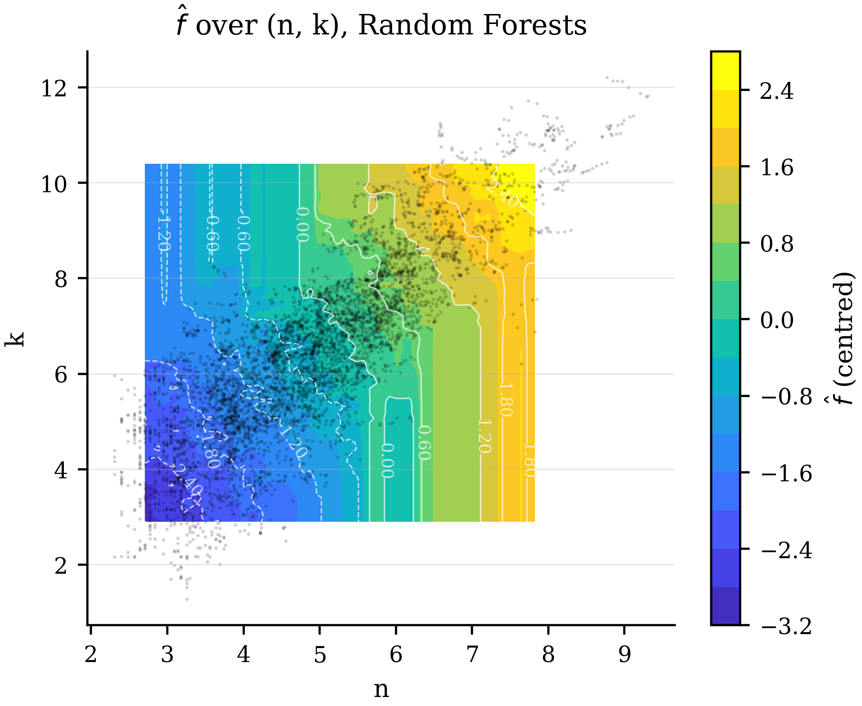
Parallel straight contours would mean Cobb–Douglas was adequate. This is the single most informative picture of what the machine learning step bought.
Specifications
spec |
$\dim z$ | Blocks | Paper's label |
|---|---|---|---|
"crfe" |
$2d+2$ | cross-sectional and time averages | CR + FE |
"fe" |
$d+1$ | time averages only | FE |
"cr" |
$d+1$ | cross-sectional averages only | addition |
"pooled" |
0 | none | Pooled |
"cr" isolates the contribution of the CCE block, which the paper's three
specifications cannot. Report more than one — the comparison is the
evidence.
Learners
The estimator is learner-agnostic: anything satisfying condition (C3), $\hat\eta-\eta = o_p((NT)^{-1/4})$, will do.
| Key | Estimator | In the paper |
|---|---|---|
"lasso" |
standardised LassoCV |
yes |
"lasso_fixed" |
Lasso with an explicit penalty, for validation-block tuning |
— |
"rf" |
RandomForestRegressor(n_estimators=500) |
yes |
"nn" |
MLPRegressor(hidden_layer_sizes=(32,16,8)) — the Gu–Kelly–Xiu architecture |
yes |
"ols" |
LinearRegression — makes the estimator analytically checkable |
— |
"ridge", "gbr", "et", "krr" |
ridge, boosting, extra trees, kernel ridge | boosting named as admissible |
Any scikit-learn regressor works, and the three stages can differ:
MLLPanel(learner="rf",       # flexible g and m — these only need to predict well
         learner_f="krr")    # smooth f — this one gets differentiated
The paper's own simulation result is a clean rule: LASSO when $f$ is sparse and linear (Tables 1, 5), forests or networks when it is not (Tables 2, 6, where LASSO hits a bias floor no amount of data fixes).
"lasso"is aLassoCVand has noalphato tune. For the paper's validation-block protocol use"lasso_fixed"withgrid={"model__alpha": ...}.
Standard errors
vcov |
Meat matrix | Use when |
|---|---|---|
"theorem1" / "hc" |
$\sum\psi\psi'$ | you want the paper's literal formula (but see above) |
"cluster_unit" |
by unit | the time-average block carries your argument |
"cluster_time" |
by period | the cross-sectional-average block carries your argument |
"twoway" |
Cameron–Gelbach–Miller, PSD-projected | default; never anti-conservative |
"dk" |
Driscoll–Kraay with Bartlett HAC | as cluster_time, with serial correlation |
Two Wald tests run automatically:
model.wald_["common_factors"]   # H0: no unobserved common factors
model.wald_["fixed_effects"]    # H0: Mundlak — effects uncorrelated with x
When a block's switch is genuinely off, its coefficients are individually unidentified (the block is collinear up to an $O_p(T^{-1/2})$ term) even though its fitted contribution is pinned at zero. Test the contribution via
productivity()["factor_part"], not a single coefficient.
Faithfulness to the paper
Every equation is mapped to the code that implements it in
THEORY.md §5.
Where the paper leaves a choice open, mllpanel picks a documented default and
exposes the alternative:
| Choice | Paper | Default here | Alternative |
|---|---|---|---|
| Fold construction | unspecified | fold_scheme="block" |
"interleaved", "random" |
| Leftover periods when $T \nmid K$ | $T_0=[T/K]$ drops them | keep them | drop_remainder=True |
| $\hat\beta$ aggregation | eq. (6), pooled | beta_agg="pooled" |
"mean" (footnote 1) |
| Second-stage $f$ | full sample | full sample | f_crossfit=True |
| Standard errors | none given | vcov="twoway" |
"theorem1" and three others |
| $R^2$ | uncentred (Gu–Kelly–Xiu) | both reported; r2_ is centred |
r2_uncentered_ |
| Forest hyper-parameters | unreported | 500 trees, sklearn defaults | tune on a validation block |
Two limitations of the method itself, documented because they bound what any implementation can deliver:
- $\beta$ is derived locally but used globally. Appendix A makes the coefficients on $\bar x_t$ and $\bar x_i$ equal $-\theta(x)$, the gradient of $f$ at the expansion point. Under a nonlinear $f$ that varies with $x$, so a constant $\beta$ is an approximation whose error goes into $e_{it}$.
- Homogeneous factor loadings are implicitly required. The coefficient on
$\bar y_t$ is $\gamma_i'(\bar\gamma\bar\gamma')^{-1}\bar\gamma$, which is
unit-specific; a pooled $\beta_1$ needs it constant. The paper's simulations
set $\gamma_i=0.5$ for every $i$, so the design never stresses this. Test it
with
simulate_panel(gamma="random").
Also documented: a short
errata list
for the published paper — most visibly, every panel of Figures 1–6 is labelled
"ISS R-Square" on the vertical axis, including Figures 1 and 2, which plot
mean squared error. This package labels axes by the quantity plotted.
Run print(mllpanel.deviations()) for the list at runtime.
Tables and figures
Journal-quality output, ready to \input into a manuscript.
- Tables use
booktabs: no vertical rules,\multicolumngroups with\cmidrule, full-width panel captions for Panels A/B/C, optional bolding of the best cell per row, and a notes block. LaTeX escaping is automatic but leaves any cell containing$alone, so$d$survives whileomega_itgets its underscore escaped. - Figures export as vector PDF with
pdf.fonttype 42, so text stays editable, plus 400 dpi PNG for slides. - Every figure uses colour and dash pattern and marker, so it survives greyscale printing.
Ten figure types: sensitivity panels (Figures 1–6), convergence, coefficient plots, partial dependence, isoquant contours, 3-D surfaces, factor paths, productivity distributions, nuisance-quality bars, dependence reports.
LaTeX preamble: \usepackage{booktabs}, plus rotating if you use
landscape=True.
Cost and performance
Each fit trains $K(1+\dim z)$ nuisance models plus one second stage — with
spec="crfe", $d=5$ and $K=5$ that is 61 model fits per estimation. Plan
accordingly.
| Task | Rough cost |
|---|---|
One crfe fit, LASSO, $N{=}738$, $T{=}8$, $d{=}2$ |
~1 s |
One crfe fit, random forest, same |
~20 s |
| Section 4 script, 3 learners + 6 benchmarks + 8 figures | ~10 min |
| Tables 1–6, 6 designs × 10 reps × 2 learners | ~15 min |
| The published grid, 72 designs × 1000 reps × 3 learners × 3 specs | days |
Levers: n_jobs= parallelises folds and Monte Carlo replications;
paper_designs(quick=True) while developing; montecarlo.estimate_runtime()
times one replication per design and extrapolates before you commit;
make_learner("rf", n_estimators=100) for a cheaper forest.
Troubleshooting
| Symptom | Cause | Fix |
|---|---|---|
RuntimeError: No candidate ... could be fitted |
"lasso" is a LassoCV with no alpha |
use "lasso_fixed" |
| $R^2$ of 0.9999 for every model | uncentred $R^2$ on log levels | report model.r2_, not r2_uncentered_ |
Coefficient on ybar_i far from 1 |
the panel does not match the model's structure, or $T$ is tiny | see GUIDE.md §8 |
Negative out-of-fold $R^2$ in nuisance_fit_ |
a $z$ column varying over few periods, extrapolated by block folds | try fold_scheme="interleaved"; see GUIDE.md §9 |
Wald test rejects but factor_part ≈ 0 |
block coefficients unidentified when the switch is off | test the contribution, not a coefficient |
Duplicate (unit, time) pairs detected |
repeated cells | aggregate or de-duplicate first |
Huge standard errors under vcov="theorem1" |
the i.i.d. plug-in is 6–16× too wide | use "twoway", or match the dimension |
singular ... using the pseudo-inverse |
a time-invariant regressor is collinear with its own time average | drop it from x, or use spec="cr" |
Forest elasticities with enormous Std. dev. |
piecewise-constant $\hat f$ | raise relative_step, or set learner_f="krr" |
predict raises on unseen units |
their time averages are unidentified | unseen_units="grand_mean", and say so |
unbalanced warning |
Appendix A assumes balance | proceed but report it |
The full 12-row version, with explanations, is in GUIDE.md §16.
Testing
pytest -q # 148 tests
The suite is not a smoke test. Under the paper's Type 1 design the whole
estimator has a closed-form answer, so
tests/test_oracle.py
checks $\hat\beta$ against the algebra of Appendix A:
- $\hat\beta$ matches $(c_2, -c_2\theta', c_1, -c_1\theta')$ to within 0.03;
- the coefficients on
ybar_tandybar_iare 1, and onxbar_i[x1..x3]are $-0.2$, with the irrelevant regressors at 0; - $MSE(f)$ orders
crfe<fe<pooledunder Panel C, with a factor of ten between the extremes, reproducing the paper's headline result; - $MSE(f)$ halves as $T$ quadruples — Theorem 2 in practice;
- with no latent terms,
pooledwins slightly, reproducing Panel A.
Also tested: every covariance estimator gives finite positive standard errors and a PSD matrix; the score is orthogonal at $\hat\beta$; folds partition the time index; the CD test detects a factor structure and accepts independence; all ten figure types build; every LaTeX table renders.
Citation
@unpublished{yang2024mlpanel,
  author = {Yang, Bingduo and Long, Wei and Cai, Zongwu},
  title  = {Machine Learning Based Panel Data Models},
  year   = {2024},
  note   = {Working paper}
}

@software{roudane2026mllpanel,
  author  = {Roudane, Merwan},
  title   = {mllpanel: Machine Learning Based Panel Data Models},
  version = {0.1.0},
  year    = {2026},
  url     = {https://github.com/merwanroudane/mllpanel}
}
Or print(mllpanel.citation("bibtex")).
License
MIT — see LICENSE.
The bundled datasets are redistributed from the R package plm under GPL-2;
their original sources are documented in src/mllpanel/datasets/_loaders.py.
Author
Dr Merwan Roudane · github.com/merwanroudane
1 maintainer

Download files
Download the file for your platform. If you're not sure which to choose, learn more about installing packages.
Source Distribution
Built Distribution
Filter files by name, interpreter, ABI, and platform.
If you're not sure about the file name format, learn more about wheel file names.
Copy a direct link to the current filters
File details
Details for the file mllpanel-0.1.0.tar.gz.
File metadata
- Download URL: mllpanel-0.1.0.tar.gz
- Upload date:
- Size: 410.9 kB
- Tags: Source
- Uploaded using Trusted Publishing? No
- Uploaded via:
twine/7.0.0 CPython/3.11.0
File hashes
| Algorithm | Hash digest | |
|---|---|---|
| SHA256 |
2f12c5e922ffc4c1bf1207ea59f22086eb3ad9daf0fa336ede72e99194a31e4f
|
|
| MD5 |
b5c4a0b530346b42c60c019ec84bc01f
|
|
| BLAKE2b-256 |
fb72b5e71e623ab030e05ebf871e75de7de1f85467f40d9f323b99c423092665
|
File details
Details for the file mllpanel-0.1.0-py3-none-any.whl.
File metadata
- Download URL: mllpanel-0.1.0-py3-none-any.whl
- Upload date:
- Size: 337.5 kB
- Tags: Python 3
- Uploaded using Trusted Publishing? No
- Uploaded via:
twine/7.0.0 CPython/3.11.0
File hashes
| Algorithm | Hash digest | |
|---|---|---|
| SHA256 |
4c082448b10024d1696831013fa7bc1b76acbbb5a9cd887a8a52bff905286b79
|
|
| MD5 |
3b0c0de4dace0dd7f9a8bdb9f6aafc01
|
|
| BLAKE2b-256 |
6ba9ce8df0207058ffaddf791473de9a4d8774cc3f90a136fb8f693a0ae08afd
|













