
MCMC samplers in Apple MLX

Project description
mlxmc
MCMC samplers written in Apple MLX, using its
grad / vmap / compile transforms. MLX has no probabilistic-programming library
yet (nothing like BlackJAX or NumPyro), so this is a first pass at one.
Status: research code. The samplers are tested (moment recovery, Σ-estimation, affine invariance, the autocorrelation diagnostics, and the convergence diagnostics validated against ArviZ, on both the CPU and Metal backends), but the API is young and likely to change. Provided as-is, no guarantees.
What's here
The package lives under src/mlxmc/; runnable demos and the benchmark study are in
examples/.
Module (mlxmc.) |
Sampler / tool |
|---|---|
ensemble |
Affine-invariant ensemble (Goodman & Weare 2010 — the emcee stretch move). Gradient-free, tuning-free. make_sampler, run_ensemble. |
hmc |
Hamiltonian Monte Carlo, identity mass. grad ∘ vmap batched over chains. make_hmc, run_hmc. |
preconditioned |
Mass-matrix HMC (M = Σ⁻¹). make_phmc, run_phmc. |
warmup |
Stan-style warmup: dual-averaging step size + windowed dense mass-matrix estimation. warmup, run_chain. |
nuts |
NUTS (multinomial; Hoffman & Gelman 2014), vectorized over chains. Reports divergences. make_nuts, run_nuts. Serial (no-vmap) variants make_nuts_serial / run_nuts_serial / nuts_warmup_serial run one chain at a time (multi-chain via a host loop) for targets MLX can't vmap over chains — e.g. a conv-net forward (Pad vmap is NYI, and conv can't batch per-chain weights). Same algorithm + Result, slower. |
result |
Result — the unified return type for every sampler: draws (chain, draw, dim), sample_stats (divergences, tree depth), .summary(), .to_arviz(). |
diagnostics |
Convergence: rank-normalized split-R̂, bulk/tail-ESS, MCSE (Vehtari et al. 2021), validated against ArviZ. Efficiency: integrated autocorrelation time + the cross-sampler ESS/sec metric. |
transforms |
Constrained-parameter bijectors (Exp, Sigmoid, …) + constrain() — sample bounded/positive parameters without hand-writing the log-Jacobian. |
targets |
Example log-densities: correlated Gaussian, banana, centered / non-centered funnel, with known moments. |
Example (examples/) |
What it shows |
|---|---|
gaussian_ess.py |
Ensemble vs identity-mass HMC vs preconditioned HMC by ESS/sec on the Gaussian. |
warmup_validation.py |
Warmup recovers the true Σ and matches oracle ESS/sec. |
hard_targets.py |
Banana + funnel benchmark (lscan / dscan modes). |
nuts_funnel.py |
NUTS correctness on the Gaussian; funnel mode for the masking-overhead study. |
affine_invariance.py |
Empirical proof of affine invariance (same RNG → bit-identical acceptance under an affine map). |
constrained_model.py |
Infer (μ, σ>0) of a Normal with a parameter transform, then Result.summary() in natural space. |
plot_hard_targets.py |
Renders hard_targets_figure.png (needs the optional viz env). |
Why MLX
grad, vmap, jvp/vjp, and compile transfer almost directly from JAX,
with JAX-style functional RNG keys (mx.random.split). The wrinkles that shape
this code:
- No traced control-flow primitives (no
while_loop/scan/cond). MLX is eager execution pluscompileof static graphs. Fixed-length unrolled loops (leapfrog, fixed-LHMC) compile fine; data-dependent trajectory length (NUTS) is the hard case —mlxmc.nutsruns every chain to a fixedmax_tree_depthand masks finished chains. - fp32 on the GPU. Apple Metal has no fp64 in hardware (MLX has fp64 only on the CPU backend). See the precision envelope below.
Numerical precision (fp32)
fp32-on-GPU is a permanent constraint, not a bug to fix, so it's worth being explicit about where it's fine and where it isn't:
- Fine (the regime this package targets): smooth, moderate-dimensional targets where
Monte Carlo error (~1/√ESS, typically 1–3%) swamps fp32 roundoff (~1e-6). All the
examples here live here. Ill-conditioned linear algebra (covariance, Cholesky in
warmup) is already kept host-side in numpy fp64; only the leapfrog runs fp32 on the GPU — generalize that pattern for any precision-sensitive sub-step. - Watch out (validate against fp64 first): large log-likelihood sums (e.g. N≳1e5 data points — roundoff accumulates and corrupts Metropolis acceptance); constrained transforms near a boundary (logit/log of values near their limit); long or stiff trajectories (deep NUTS trees). For these, run the CPU fp64 backend to check, or sum in fp64 host-side.
The defensible niche is fp32-tolerant, memory-bound, differentiable/stochastic work — not fp64-precision HPC.
Install
This is a pixi project (installs the package editable):
pixi install
pixi run python examples/gaussian_ess.py             # ensemble vs HMC vs preconditioned
pixi run python examples/nuts_funnel.py funnel        # several examples have demo modes
pixi run -e viz python examples/plot_hard_targets.py  # plotting needs the optional viz env
Or install into any environment with pip: pip install -e . (needs mlx, so arm64
macOS). Add the plotting extra with pip install -e ".[viz]" (matplotlib).
Usage
Every sampler takes a single-point log-density logp(x) -> scalar for x of
shape (D,); batching over walkers/chains is handled internally with vmap.
Positions are MLX arrays of shape (n_chains, D).
import mlx.core as mx
import numpy as np

# Target: a strongly correlated 2-D Gaussian (corr 0.9, 25:1 variance ratio).
# mlxmc.targets ships this one (as `gaussian_logp`) plus banana / funnel.
mu = mx.array([1.0, -2.0])
Sig_inv = mx.array(np.linalg.inv([[25.0, 4.5], [4.5, 1.0]]))

def logp(x):                              # x: (D,) -> scalar
    d = x - mu
    return -0.5 * (d @ Sig_inv @ d)

key = mx.random.key(0)
Gradient-free ensemble — no tuning, handles the ill-conditioning for free:
from mlxmc import run_ensemble

key, k = mx.random.split(key)
ensemble = mx.random.normal(shape=(2000, 2), key=k) * 5.0     # (n_walkers, D)
result = run_ensemble(logp, ensemble, n_steps=3000, burn=1000, key=key)
print(result.accept_frac)
result.summary()                                             # mean / sd / mcse / ESS / R̂
HMC, hand-tuned, and NUTS after Stan-style warmup (same logp):
from mlxmc import run_hmc, warmup, run_nuts

key, k = mx.random.split(key)
q0 = mx.random.normal(shape=(1000, 2), key=k) * 5.0           # (n_chains, D)

result = run_hmc(logp, q0, n_steps=1500, burn=500, eps=0.15, n_leap=40, key=key)

# Warmup adapts (eps, dense M); NUTS then adapts trajectory length itself.
q_last, eps, Minv = warmup(logp, q0, n_warmup=600, n_leap=8, key=key)
result = run_nuts(logp, q_last, n_samples=1500, eps=eps, Minv_np=Minv, key=key)
print("divergences:", result.n_divergent)                    # NUTS surfaces these now
result.summary()
Every sampler returns a
Result.result.samplesis(chain, draw, dim),result.flatpools to(chain·draw, dim),result.accept_fracis the acceptance, andresult.sample_statscarries per-drawdiverging/tree_depth(NUTS).result.summary()prints rank-normalized split-R̂, bulk/tail-ESS, and MCSE per parameter;result.to_arviz()hands off to ArviZ (pip install 'mlxmc[arviz]') for the full plotting/diagnostic suite. The warmup helpers (warmup,nuts_warmup) instead return the tuning triple(q_last, eps, Minv).
Constrained parameters — sample positive / bounded parameters without writing a
Jacobian by hand (see examples/constrained_model.py):
from mlxmc import Transform, Identity, Exp, constrain, run_nuts

def logp_constrained(theta):          # theta = (mu, sigma > 0)
    mu, sigma = theta[0], theta[1]
    return -0.5 * (((data - mu) / sigma) ** 2).sum() - data.shape[0] * mx.log(sigma)

# mu free, sigma positive; constrain() adds the log-Jacobian so you sample in R^2.
logp_u, transform = constrain(logp_constrained, Transform([Identity(), Exp()]))
result = run_nuts(logp_u, u0, n_samples=1000, eps=eps, Minv_np=Minv, key=key)
result.transform = transform          # map draws back to natural (mu, sigma) space
result.summary()                      # reported in constrained space
natural_draws = result.constrained()
Findings
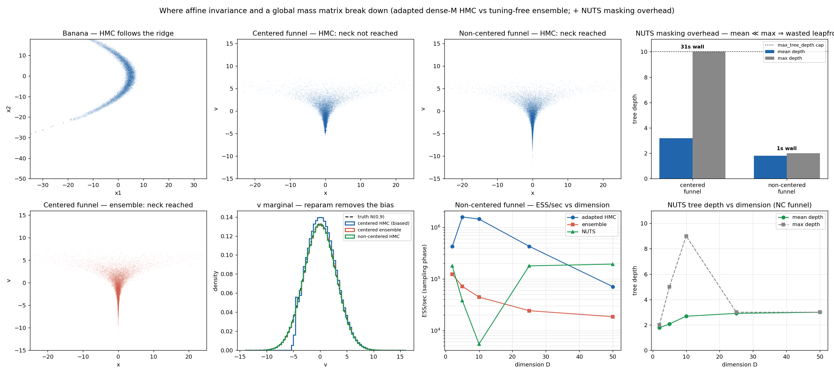
Validated on a corr-0.9, 25:1-variance Gaussian and on banana / funnel targets;
every number below is reproducible with the scripts in
examples/:
- Affine-invariant ensemble is the robust low-D default: gradient-free, tuning-free, handles ill-conditioning for free (acceptance is bit-identical under an affine map). But weaker per-step mixing and it degrades with dimension.
- HMC needs gradients and a tuned
eps/L, but mixes far better (τ≈2 vs ≈26). A warmup-adapted dense mass matrix recovers the true Σ to <1% Frobenius error and buys ~7–11× the ESS/sec — HMC's version of affine invariance, earned rather than supplied. - Fixed-
LHMC has a trajectory resonance: on near-Gaussian targets, wheneps·Llands near a multiple of 2π the trajectory returns to its start and mixing collapses. Jitteringepsper trajectory cures it; NUTS's adaptive trajectory length is the principled fix. - NUTS is validated exact on the Gaussian (recovered covariance 24.97 vs 25)
and auto-tunes trajectory length, but vectorized NUTS pays a real masking cost
when trajectory lengths are heterogeneous — with no
while_loop, every chain runs to the deepest chain's tree depth, up to a ~30× wall-time penalty at the funnel mouth versus the same target reparametrized. - Geometry matters more than the sampler: on the centered funnel the gradient-free ensemble beats a global-metric HMC, because a constant mass matrix is wrong everywhere when the scale is position-dependent; a non-centered reparametrization removes the geometry and makes HMC unbiased again.
- ESS/sec is the honest efficiency metric — acceptance fraction is a misleading proxy.
Development
pixi run test                                   # full suite on the default device
MLXMC_TEST_DEVICE=cpu pixi run test             # force the CPU backend
MLXMC_TEST_DEVICE=gpu pixi run test             # force the Metal GPU
pixi run -e dev test                            # incl. the ArviZ-validated diagnostics tests
The suite (tests/) checks moment recovery for every sampler, warmup's Σ
estimate, the affine-invariance identity, the autocorrelation-time diagnostics,
divergence reporting, the constrained-parameter transforms, and the convergence
diagnostics (R̂ / bulk-tail-ESS / MCSE) against ArviZ. The ArviZ comparison needs
arviz + scipy, which live in the optional dev pixi environment (run those via
pixi run -e dev test); they're skipped in the lean default env. A GitHub Actions
workflow (.github/workflows/tests.yml) runs the
CPU + GPU matrix on an Apple-silicon runner for pull requests to main (and on
manual dispatch from the Actions tab). Direct pushes to main don't trigger it,
which keeps the (10x-billed) macOS runner minutes down.
References
- Goodman & Weare (2010), Ensemble samplers with affine invariance.
- Hoffman & Gelman (2014), The No-U-Turn Sampler.
- Betancourt (2017), A Conceptual Introduction to Hamiltonian Monte Carlo.
License
Release history Release notifications | RSS feed


Download files
Download the file for your platform. If you're not sure which to choose, learn more about installing packages.
Source Distribution
Built Distribution
Filter files by name, interpreter, ABI, and platform.
If you're not sure about the file name format, learn more about wheel file names.
Copy a direct link to the current filters
File details
Details for the file mlxmc-0.3.0.tar.gz.
File metadata
- Download URL: mlxmc-0.3.0.tar.gz
- Upload date:
- Size: 421.7 kB
- Tags: Source
- Uploaded using Trusted Publishing? No
- Uploaded via: twine/6.2.0 CPython/3.14.5
File hashes
| Algorithm | Hash digest | |
|---|---|---|
| SHA256 |
38b3a177fdbbf2cdcd5aff542582587ffcb8792209ef7675df270b5c7b653a27
|
|
| MD5 |
6473ea15a3be30e55f327531c7264d86
|
|
| BLAKE2b-256 |
529b9ae57f6e7bc08c2d193b4dd59c1a3a5776afe9e9ee81c8040f9e396ef2ae
|
File details
Details for the file mlxmc-0.3.0-py3-none-any.whl.
File metadata
- Download URL: mlxmc-0.3.0-py3-none-any.whl
- Upload date:
- Size: 33.1 kB
- Tags: Python 3
- Uploaded using Trusted Publishing? No
- Uploaded via: twine/6.2.0 CPython/3.14.5
File hashes
| Algorithm | Hash digest | |
|---|---|---|
| SHA256 |
723d41e49c4d26a366acfe61eb9c0c39e6579f316abd1cc4ebd45bc577183584
|
|
| MD5 |
78fac44deb32aee21a49a3e14c45a992
|
|
| BLAKE2b-256 |
c97564184f44a6c5b6bc2c6e0a0aa79db942a000c2cd1624da1e1c3af278eccb
|






