




NanoPlaceR: Reinforcement-learning placement and routing for FCN

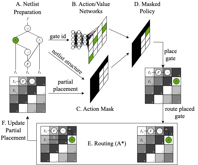
NanoPlaceR is an open-source physical-design tool for field-coupled nanocomputing (FCN). It uses masked Proximal Policy Optimization to place logic elements and routes each partial placement with A* search. It can generate layouts for logic networks of roughly 200 gates while using about 50% less area than the state-of-the-art heuristic approach described in the publications below.
Installation
NanoPlaceR supports Python 3.11 through 3.14 and requires mnt.pyfiction 0.8 or newer. The CI suite covers both ends of that range.
python -m venv .venv
source .venv/bin/activate
python -m pip install mnt.nanoplacer
On Windows, activate the environment with .venv\Scripts\activate.
Usage
Use NanoPlaceR from Python:
from mnt.nanoplacer import create_layout

create_layout(
    benchmark="trindade16",
    function="mux21",
    clocking_scheme="2DDWave",
    technology="QCA",
    minimal_layout_dimension=False,
    layout_width=3,
    layout_height=4,
    time_steps=None,  # Automatic network-size budget; set an integer to override.
    reset_model=True,
    verbose=1,
    optimize=True,
    seed=42,
    stop_on_solution=True,
)
Or use the command-line interface:
mnt.nanoplacer --help
mnt.nanoplacer --benchmark trindade16 --function mux21 \
  --clocking-scheme 2DDWave --technology Gate-level \
  --minimal-layout-dimension --seed 42 --verbose 1
Runs store generated layouts in layouts/, trained agents in models/, and TensorBoard data in tensorboard/. By default, the CLI resumes a matching saved model when one exists; pass --reset-model to train from scratch.
Pass --stop-on-solution (or stop_on_solution=True in Python) to stop after the first equivalent layout and save the checkpoint. Otherwise training continues, retaining equivalent solutions that improve area, then wire count, then crossing count. Complete candidates are checked for equivalence before they can replace solution exports. Both strong and weak equivalence count as verified; weak equivalence permits different timing. This does not change the agent's reward function.
Browser interface
Install the optional standalone GUI and launch it locally:
python -m pip install "mnt.nanoplacer[gui]"
mnt.nanoplacer.gui
The interface opens at http://127.0.0.1:5056. Use --port 5057 to choose another port, --no-browser to suppress automatic opening, or --runs-dir PATH to choose where experiments are saved.
Choose a bundled circuit, technology and clocking scheme, then configure its grid, random seed and training budget. The canvas shows the best partial placement, including the actual clock phases; complete candidates and verified solutions are identified separately. SiDB uses 2DDWave during training and converts its output to a hexagonal layout. Optimization is available for 2DDWave only. Predefined minimum dimensions are experimental targets, not a guarantee that every seed or budget will find a solution.
The GUI, Python API, and CLI default to 1,000 timesteps per placement node, with a 10,000-step minimum and a 10-million-step cap. The count includes inputs, outputs, and fanout nodes after substitution: mux21 has 9 nodes (10,000 steps), while fontes18/parity has 150 (150,000 steps). This is a size-based starting heuristic, not a measured minimum or a guarantee of success. Uncheck Automatic timestep budget in the GUI, pass time_steps in Python, or use --time-steps on the CLI to set your own budget. Saved runs retain their exact resolved budget. The GUI rejects grids with fewer tiles than placement nodes; additional space is usually needed for routing.
GUI circuit sizing runs in a separate process with a 10-second timeout and caches successful results, keeping status and Stop controls responsive even while a large circuit is being parsed. Circuits with constant-driven gates or outputs (including ISCAS85/c2670) are currently unsupported and are rejected before training starts, rather than failing partway through placement.
Training runs in a separate process, one run at a time per GUI instance. Select up to ten consecutive seeds to test the same dimensions with independent fresh agents. The timestep budget applies to each seed, and seeds run sequentially. Stop cancels the active run and the remaining queue, requesting a graceful checkpoint save; if a native operation prevents that, the worker is terminated after a short grace period. A finished training budget without a solution is reported honestly as such. PPO may finish its current rollout beyond the requested timestep budget.
Run history lets you inspect previous results and compare seeds, layout quality, and time to a verified solution while another experiment continues. You can repeat a run's settings without changing its saved files. History survives a server restart; interrupted work is not automatically restarted. The training statistics panel plots the mean return of the latest 100 completed episodes (fewer at the start), with sampled history and timesteps relative to the current run. Separate quality metrics show dimensions before and after optimization, wires, crossings, and verified episode counts: reward itself is not an independent quality score.
Comparison can be restricted to matching circuit, clocking, technology, grid, budget, optimization, stopping, and fresh/resumed settings. Recorded circuit hashes, software versions, and source checkpoints keep different experiment conditions separate. The table shows requested and actual timesteps. Seed summaries count distinct seeds from completed fresh runs; repeated seeds, resumed runs, failures, cancellations, and unfinished runs are identified separately rather than pooled into an apparent success rate.
For new runs, Reported target reproduced requires a verified layout on the exact reported width and height before post-layout optimization. The unoptimized proof is saved as *_reported_target.fgl; a smaller optimized layout obtained from a different starting grid does not establish this result. Older runs without this evidence are marked unknown. Learning statistics also show best placement progress and PPO training epochs, both for this run and over the checkpoint's lifetime. These epochs are not individual optimizer steps. A fresh agent can find a solution before any PPO training has occurred; the first-solution timestep and epoch count make that distinction visible. Episode success is measured during training, not on an independent evaluation set.
Replay shows up to 128 sampled best-placement improvements, not every action or episode. Its immutable milestones can be inspected with a slider or played back; Live always returns to the latest best layout, even after recording reaches its limit. Expand the canvas for inspection or export a lossless PNG of the full layout, independent of the current pan and zoom.
Each run has its own folder under nanoplacer-runs/, with configuration, a reproducibility manifest, log, previews, generated layouts and a saved agent. The manifest records the Python/package versions, circuit hash, and source checkpoint identity and hash when resuming. Downloads become available when the worker stops writing its outputs: individual layouts/models, sampled reward CSV, metadata, or an experiment ZIP. A seed and manifest help reproduce experiments, but do not guarantee identical results across different software versions or hardware.
Continue this run copies a checkpoint from the selected experiment into a new run. Set the additional timestep budget and press Start; the source files stay unchanged. The general resume option still selects the latest compatible agent when no source run is specified. Circuit, technology, clocking scheme and grid size must match; changed circuit hashes or software versions produce a warning. Multi-seed experiments always start fresh. Only checkpoints in local run folders are accepted; never add untrusted model files to them.
During GUI training, one models/recovery.zip is atomically replaced approximately every 60 seconds, and a final checkpoint is saved on normal completion or graceful cancellation. A failed or interrupted save leaves the previous checkpoint intact. Long native operations can delay recovery saves, and resumption starts a new episode rather than replaying an interrupted rollout exactly. Checkpoint status and save failures are shown in the interface. Gate-level FGL output is also kept for verified solutions alongside the selected technology's usual output. Downloaded layouts can be opened in other MNT tools where their topology and clocking scheme are supported. Old run folders remain readable, but metrics or replay frames not recorded by earlier versions are unavailable.
This is a local workstation interface, bound to loopback, not a multi-user hosted service. It supports bundled benchmarks, grids up to 128 × 128, and budgets up to 10 million timesteps. The Python API and original CLI remain available without the GUI dependency.
Repository structure
src/mnt/nanoplacer/
├── benchmarks/                  Verilog benchmark circuits
├── main.py                      Python and command-line entry point
└── placement_envs/
    ├── nano_placement_env.py    Gymnasium placement environment
    └── utils/
        ├── layout_dimensions.py Predefined minimal dimensions
        └── placement_utils.py   Network and action helpers
tests/                           Unit and integration tests
Search-performance experiments
Routing retries skip the current unrouted gate when checking whether already placed gates can still reach their destinations. Output masks also retain reachable border positions when their source lies on row or column zero. These correctness fixes can change search trajectories compared with older versions.
The environment reuses the current action-mask count when starting a routing attempt, avoiding a second feasibility scan of the same placement. Masks are still recalculated for every policy request; routing paths are not cached across layout changes. Mask-count reuse does not alter rewards, observations, or routing order.
To try routing the other input first when a two-input route is blocked, pass routing_fallback=True to create_layout, or --routing-fallback to the CLI. This is an opt-in experiment, not a guarantee of smaller layouts: the extra routing attempts can also cost time. Its checkpoints and TensorBoard logs are separate from normal runs. The browser interface keeps the default routing behavior.
The repository includes a paired benchmark using the usual PPO settings:
python scripts/benchmark_search.py --baseline-ref 80892fd --trace-steps 0 \
  --circuits trindade16/mux21 fontes18/cm82a_5 \
  --seeds 42 43 44 --seconds 30 --output /tmp/nanoplacer-benchmark
It compares fresh, single-CPU-thread runs at equal wall-clock budgets. Results include dependency versions, source identity, throughput, verified layout quality, and actual deadline overruns. Run it on an otherwise idle machine. The baseline must be a trusted local Git revision; the comparison loads its environment implementation using the current checkout's utilities. The baseline at 80892fd predates routing/mask correctness fixes and retains only its first complete candidate, so neither identical trajectories nor best-of-every-episode quality is expected. Use --trace-steps 0 for comparisons where search behavior intentionally differs. For behavior-preserving changes, omit that option to check identical masked-action trajectories; version-specific diagnostic fields are ignored, but observation, reward, termination, and layout differences still fail the check. Reward-shaping experiments are not enabled by this change.
To benchmark the routing experiment, add --routing-fallback --trace-steps 0. This changes the search, so identical-trajectory checks do not apply.
References
If you use NanoPlaceR in your work, please cite the following publications:
- Late Breaking Results From Hybrid Design Automation for Field-coupled Nanotechnologies (DAC 2023)
- Thinking Outside the Clock: Physical Design for Field-coupled Nanocomputing with Deep Reinforcement Learning (ISQED 2024)
@INPROCEEDINGS{hofmann2023nanoplacer,
  author        = {S. Hofmann and M. Walter and L. Servadei and R. Wille},
  title         = {{Late Breaking Results From Hybrid Design Automation for Field-coupled Nanotechnologies}},
  booktitle     = {{2023 60th ACM/IEEE Design Automation Conference (DAC)}},
  year          = {2023},
}
@INPROCEEDINGS{hofmann2024nanoplacer,
  author        = {S. Hofmann and M. Walter and L. Servadei and R. Wille},
  title         = {{Thinking Outside the Clock: Physical Design for Field-coupled Nanocomputing with Deep Reinforcement Learning}},
  booktitle     = {{2024 25th International Symposium on Quality Electronic Design (ISQED)}},
  year          = {2024},
}
1 maintainer

Metadata
1 maintainer
Release files for mnt.nanoplacer 0.3.1
For a detailed explanation of source distributions (sdists) and built distributions (wheels), please see the package formats documentation.
Source distribution (sdist)
| File | Size | Uploaded | |
|---|---|---|---|
| mnt_nanoplacer-0.3.1.tar.gz | 4.3 MB | Details |
Built distribution (wheel)
| File | Interpreter | ABI | Platform | Reset |
|---|---|---|---|---|
| mnt_nanoplacer-0.3.1-py3-none-any.whl | Python 3 | none | any | Details |
Total release size: 8.6 MB
Release files / mnt_nanoplacer-0.3.1.tar.gz
| Download URL | mnt_nanoplacer-0.3.1.tar.gz |
|---|---|
| Size | 4.3 MB |
| Tags | Source |
|
SHA-256 checksum How to use checksums |
75374de5fb5052f8dd36e36b33a46cc398023d015f315eae714676d6190ff407
|
|
BLAKE2b-256 checksum How to use checksums |
49ca1afd879b8f6c1ee3cba84fe0446a80d5de6d06272aa4c2a347251344a117
|
| Upload date | |
|
Uploaded using Trusted Publishing? What is trusted publishing? |
Yes |
| Uploaded via |
twine/7.0.0 CPython/3.13.14
|
Provenance
Provenance describes where a file came from. On PyPI, provenance is shared via attestations, which provide a verifiable record of the build or publishing details. View details, limitations and caveats.


PyPI Publish Attestation
PyPI verified that this artifact, at this checksum, originated from the publisher listed below.
Signed by GitHub Actions, verified by PyPI on Sep 15, 2026.
Transparency logRelease files / mnt_nanoplacer-0.3.1-py3-none-any.whl
| Download URL | mnt_nanoplacer-0.3.1-py3-none-any.whl |
|---|---|
| Size | 4.3 MB |
| Tags | Python 3 |
|
SHA-256 checksum How to use checksums |
cbe2d262b78f1dab0d1763f4416c8c951eadb44b601232332602c63a59948fdb
|
|
BLAKE2b-256 checksum How to use checksums |
e103286ad977efa32dbf36733684c0c5d256d25a608a251383ddd6652522dbdf
|
| Upload date | |
|
Uploaded using Trusted Publishing? What is trusted publishing? |
Yes |
| Uploaded via |
twine/7.0.0 CPython/3.13.14
|
Provenance
Provenance describes where a file came from. On PyPI, provenance is shared via attestations, which provide a verifiable record of the build or publishing details. View details, limitations and caveats.
PyPI Publish Attestation
PyPI verified that this artifact, at this checksum, originated from the publisher listed below.
Signed by GitHub Actions, verified by PyPI on Sep 15, 2026.
Transparency log













