
Constrained Monotonic Neural Networks
Running in Google Colab
You can execute this interactive tutorial in Google Colab by clicking the button below:

Summary
This Python library implements Constrained Monotonic Neural Networks as described in:
Davor Runje, Sharath M. Shankaranarayana, “Constrained Monotonic Neural Networks”, in Proceedings of the 40th International Conference on Machine Learning, 2023. [PDF].
Abstract
Wider adoption of neural networks in many critical domains such as finance and healthcare is being hindered by the need to explain their predictions and to impose additional constraints on them. Monotonicity constraint is one of the most requested properties in real-world scenarios and is the focus of this paper. One of the oldest ways to construct a monotonic fully connected neural network is to constrain signs on its weights. Unfortunately, this construction does not work with popular non-saturated activation functions as it can only approximate convex functions. We show this shortcoming can be fixed by constructing two additional activation functions from a typical unsaturated monotonic activation function and employing each of them on the part of neurons. Our experiments show this approach of building monotonic neural networks has better accuracy when compared to other state-of-the-art methods, while being the simplest one in the sense of having the least number of parameters, and not requiring any modifications to the learning procedure or post-learning steps. Finally, we prove it can approximate any continuous monotone function on a compact subset of $\mathbb{R}^n$.
Citation
If you use this library, please cite:
@inproceedings{runje2023,
  title={Constrained Monotonic Neural Networks},
  author={Davor Runje and Sharath M. Shankaranarayana},
  booktitle={Proceedings of the 40th {International Conference on Machine Learning}},
  year={2023}
}
Python package
This package contains an implementation of our Monotonic Dense Layer
MonoDense
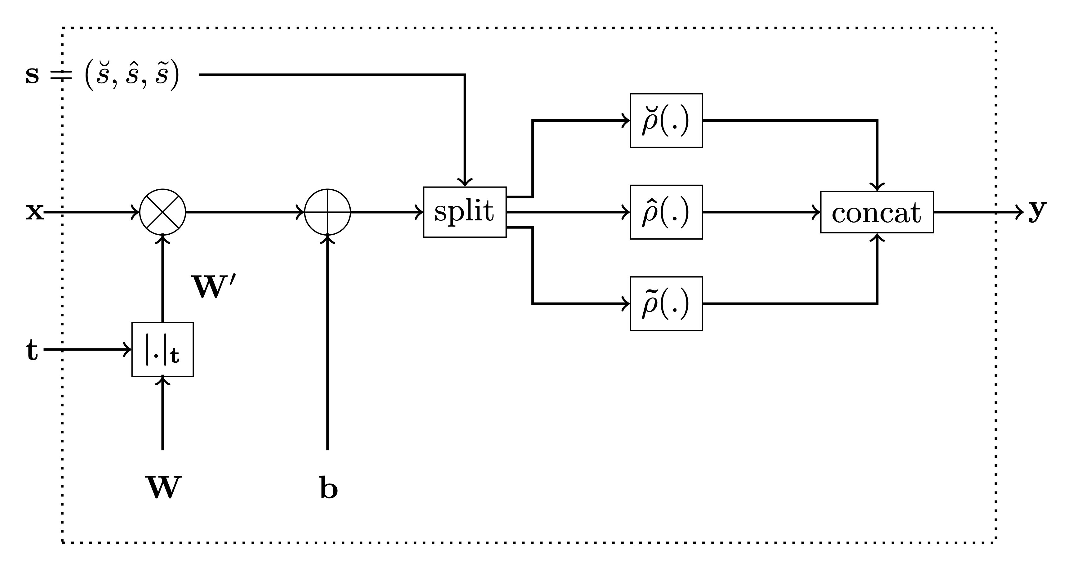
(Constrained Monotonic Fully Connected Layer). Below is the figure from
the paper for reference.
In the code, the variable monotonicity_indicator corresponds to t
in the figure and parameters is_convex, is_concave and
activation_weights are used to calculate the activation selector s
as follows:
-
if
is_convexoris_concaveis True, then the activation selector s will be (units, 0, 0) and (0,units, 0), respecively. -
if both
is_convexoris_concaveis False, then theactivation_weightsrepresent ratios between $\breve{s}$, $\hat{s}$ and $\tilde{s}$, respecively. E.g. ifactivation_weights = (2, 2, 1)andunits = 10, then
$$ (\breve{s}, \hat{s}, \tilde{s}) = (4, 4, 2) $$
Install
pip install monotonic-nn
How to use
In this example, we’ll assume we have a simple dataset with three inputs values $x_1$, $x_2$ and $x_3$ sampled from the normal distribution, while the output value $y$ is calculated according to the following formula before adding Gaussian noise to it:
$y = x_1^3 + \sin\left(\frac{x_2}{2 \pi}\right) + e^{-x_3}$
| x0 | x1 | x2 | y |
|---|---|---|---|
| 0.304717 | -1.039984 | 0.750451 | 0.234541 |
| 0.940565 | -1.951035 | -1.302180 | 4.199094 |
| 0.127840 | -0.316243 | -0.016801 | 0.834086 |
| -0.853044 | 0.879398 | 0.777792 | -0.093359 |
| 0.066031 | 1.127241 | 0.467509 | 0.780875 |
Now, we’ll use the
MonoDense
layer instead of Dense layer to build a simple monotonic network. By
default, the
MonoDense
layer assumes the output of the layer is monotonically increasing with
all inputs. This assumtion is always true for all layers except possibly
the first one. For the first layer, we use monotonicity_indicator to
specify which input parameters are monotonic and to specify are they
increasingly or decreasingly monotonic:
-
set 1 for increasingly monotonic parameter,
-
set -1 for decreasingly monotonic parameter, and
-
set 0 otherwise.
In our case, the monotonicity_indicator is [1, 0, -1] because $y$
is:
-
monotonically increasing w.r.t. $x_1$ $\left(\frac{\partial y}{x_1} = 3 {x_1}^2 \geq 0\right)$, and
-
monotonically decreasing w.r.t. $x_3$ $\left(\frac{\partial y}{x_3} = - e^{-x_2} \leq 0\right)$.
from tensorflow.keras import Sequential
from tensorflow.keras.layers import Dense, Input

from airt.keras.layers import MonoDense

model = Sequential()

model.add(Input(shape=(3,)))
monotonicity_indicator = [1, 0, -1]
model.add(
    MonoDense(128, activation="elu", monotonicity_indicator=monotonicity_indicator)
)
model.add(MonoDense(128, activation="elu"))
model.add(MonoDense(1))

model.summary()
Model: "sequential"
_________________________________________________________________
 Layer (type)                Output Shape              Param #
=================================================================
 mono_dense (MonoDense)      (None, 128)               512

 mono_dense_1 (MonoDense)    (None, 128)               16512

 mono_dense_2 (MonoDense)    (None, 1)                 129

=================================================================
Total params: 17,153
Trainable params: 17,153
Non-trainable params: 0
_________________________________________________________________
Now we can train the model as usual using Model.fit:
from tensorflow.keras.optimizers import Adam
from tensorflow.keras.optimizers.schedules import ExponentialDecay

lr_schedule = ExponentialDecay(
    initial_learning_rate=0.01,
    decay_steps=10_000 // 32,
    decay_rate=0.9,
)
optimizer = Adam(learning_rate=lr_schedule)
model.compile(optimizer=optimizer, loss="mse")

model.fit(
    x=x_train, y=y_train, batch_size=32, validation_data=(x_val, y_val), epochs=10
)
Epoch 1/10
313/313 [==============================] - 3s 5ms/step - loss: 9.4221 - val_loss: 6.1277
Epoch 2/10
313/313 [==============================] - 1s 4ms/step - loss: 4.6001 - val_loss: 2.7813
Epoch 3/10
313/313 [==============================] - 1s 4ms/step - loss: 1.6221 - val_loss: 2.1111
Epoch 4/10
313/313 [==============================] - 1s 4ms/step - loss: 0.9479 - val_loss: 0.2976
Epoch 5/10
313/313 [==============================] - 1s 4ms/step - loss: 0.9008 - val_loss: 0.3240
Epoch 6/10
313/313 [==============================] - 1s 4ms/step - loss: 0.5027 - val_loss: 0.1455
Epoch 7/10
313/313 [==============================] - 1s 4ms/step - loss: 0.4360 - val_loss: 0.1144
Epoch 8/10
313/313 [==============================] - 1s 4ms/step - loss: 0.4993 - val_loss: 0.1211
Epoch 9/10
313/313 [==============================] - 1s 4ms/step - loss: 0.3162 - val_loss: 1.0021
Epoch 10/10
313/313 [==============================] - 1s 4ms/step - loss: 0.2640 - val_loss: 0.2522

<keras.callbacks.History>
License
This
work is licensed under a
Creative
Commons Attribution-NonCommercial-ShareAlike 4.0 International
License.

You are free to:
-
Share — copy and redistribute the material in any medium or format
-
Adapt — remix, transform, and build upon the material
The licensor cannot revoke these freedoms as long as you follow the license terms.
Under the following terms:
-
Attribution — You must give appropriate credit, provide a link to the license, and indicate if changes were made. You may do so in any reasonable manner, but not in any way that suggests the licensor endorses you or your use.
-
NonCommercial — You may not use the material for commercial purposes.
-
ShareAlike — If you remix, transform, or build upon the material, you must distribute your contributions under the same license as the original.
-
No additional restrictions — You may not apply legal terms or technological measures that legally restrict others from doing anything the license permits.


Release files for monotonic-nn 0.3.5
For a detailed explanation of source distributions (sdists) and built distributions (wheels), please see the package formats documentation.
Source distribution (sdist)
| File | Size | Uploaded | |
|---|---|---|---|
| monotonic-nn-0.3.5.tar.gz | 28.2 kB | Details |
Built distribution (wheel)
| File | Interpreter | ABI | Platform | Reset |
|---|---|---|---|---|
| monotonic_nn-0.3.5-py3-none-any.whl | Python 3 | none | any | Details |
Total release size: 53.3 kB
Release files / monotonic-nn-0.3.5.tar.gz
| Download URL | monotonic-nn-0.3.5.tar.gz |
|---|---|
| Size | 28.2 kB |
| Tags | Source |
|
SHA-256 checksum How to use checksums |
6175d5df60541dfcbf759f9ede05fe526a5e44991aa2481b8f032994fc834187
|
|
BLAKE2b-256 checksum How to use checksums |
ad825e88afec2e5993ae661fd6138d8f050476dd875ee2aa30d87021abbafc8d
|
| Upload date | |
|
Uploaded using Trusted Publishing? What is trusted publishing? |
No |
| Uploaded via |
twine/6.1.0 CPython/3.9.21
|
Release files / monotonic_nn-0.3.5-py3-none-any.whl
| Download URL | monotonic_nn-0.3.5-py3-none-any.whl |
|---|---|
| Size | 25.2 kB |
| Tags | Python 3 |
|
SHA-256 checksum How to use checksums |
44da64331c44fd7ab747833c4ff4f865b09bedc1b41794004d20b709e6c2b9f3
|
|
BLAKE2b-256 checksum How to use checksums |
d86e74a714c967ea4441802c1b4d2bd840d3692156c48f530f3a175ba41b92e3
|
| Upload date | |
|
Uploaded using Trusted Publishing? What is trusted publishing? |
No |
| Uploaded via |
twine/6.1.0 CPython/3.9.21
|














