A machine learning tool to segment organoids.

Project description

MOrgAna
Welcome to MOrgAna (Machine-learning based Organoids Analysis) to segment and analyse 2D multi-channel images of organoids, as described in the paper:
Nicola Gritti, Jia Le Lim, Kerim Anlaş, David Oriola, Mallica Pandya, Germaine Aalderink, Guillermo Martinez Ara, Vikas Trivedi. MOrgAna: accessible quantitative analysis of organoids with machine learning. Development (2021) 148 (18): dev199611. https://doi.org/10.1242/dev.199611
Overview
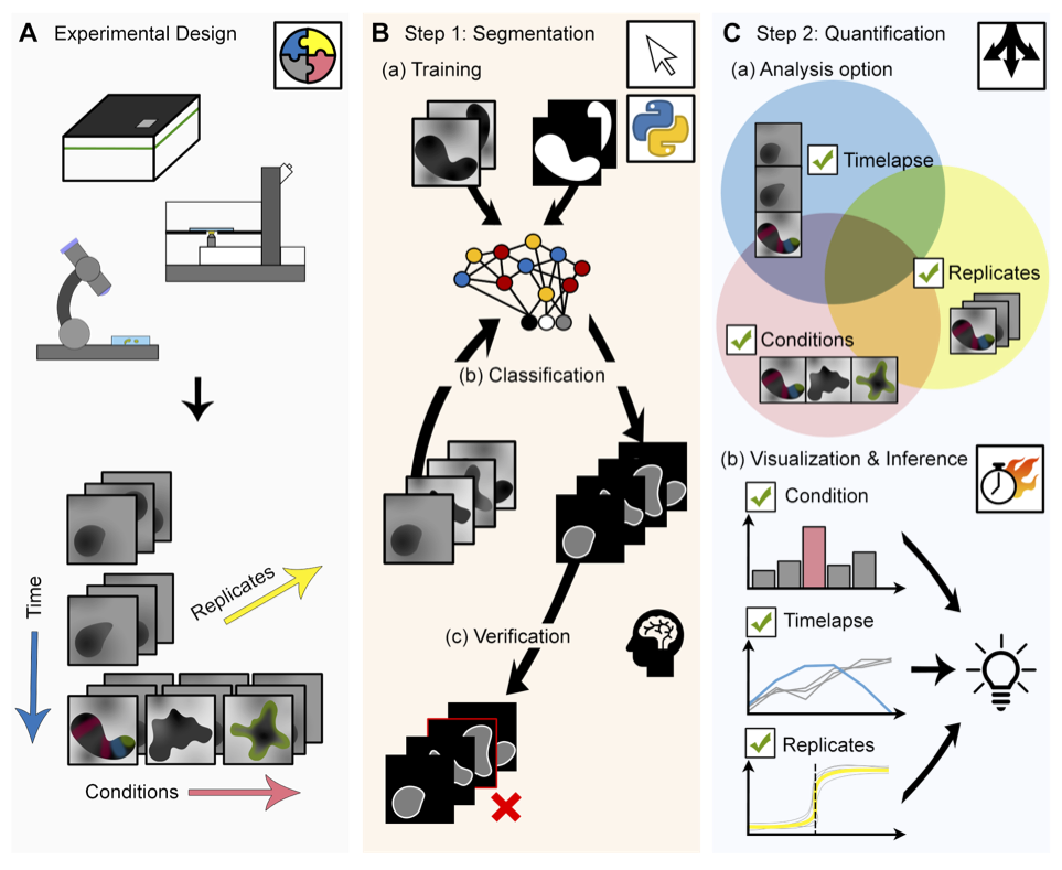
MOrgAna accepts images acquired by diverse devices such as high content screening devices, confocal microscopes and simple benchtop stereo-microscopes, trains a segmentation network based on a few manually created binary mask for the generation of addition masks of unseen images, and produces quantitative plots based on morphological and fluorescence parameters based on the input images and generated masks.
Installation
The MOrgAna software has been tested with Python 3.6 and above. To install Python, we recommend using the software Anaconda. Anaconda provides a Python distribution for Windows, Linux, and MacOS, and contains most of the pacakges used by MOrgAna.
Users can also choose to create a Conda environment using the environment_morgana.yml file found in the repository:morgana/environment_morgana.yml. To create the environment and activate it, set working directory in the MOrgAna folder and run the command conda env create -f environment_morgana.yml in terminal (MacOS) or command prompt(windows).
If problems were encountered due to package incompatibility, we recommend the use of conda or pip to perform an update of the python package.
Optional: To use deep machine learning in generation of masks, please first install TensorFlow 2 with GPU support. The tensorflow package can be installed with the command pip install tensorflow in terminal (MacOS) or command prompt(windows). Otherwise, please follow the official instructions for installation of tensorflow here.
To download the software, run pip install morgana in terminal (MacOS) or command prompt(windows).
Using the software
This software is able to A) generate binary masks of organoids based on their bright-field images and with this mask, extract morphological information, generate a midline and a meshgrid. B) Provide analysis of fluorescence signals along the generated midline and enable quick and easy visual comparisons between conditions.
To run MOrgAna, run python -m morgana in terminal (MacOS) or command prompt(windows).
For advance python users looking to analyse multiple image folders at once, please refer to the jupyter notebook morgana/Examples/MOrgAna_workflow_for_advance_python_users.ipynb.
A) Generate or Import Masks Tab
Each tif file in image folder should contain only one organoid with the brightfield channel as the starting image of each tif. Input tif files for MOrgAna can be generated from individual tif images with the use of the IJ macro morgana/Examples/IJ_macro/transform_into_stacks.ijm. Instructions for the use of the macro can be found in morgana/Examples/IJ_macro/README_transform_into_stacks.txt.
Creating binary masks
-
Manually create a
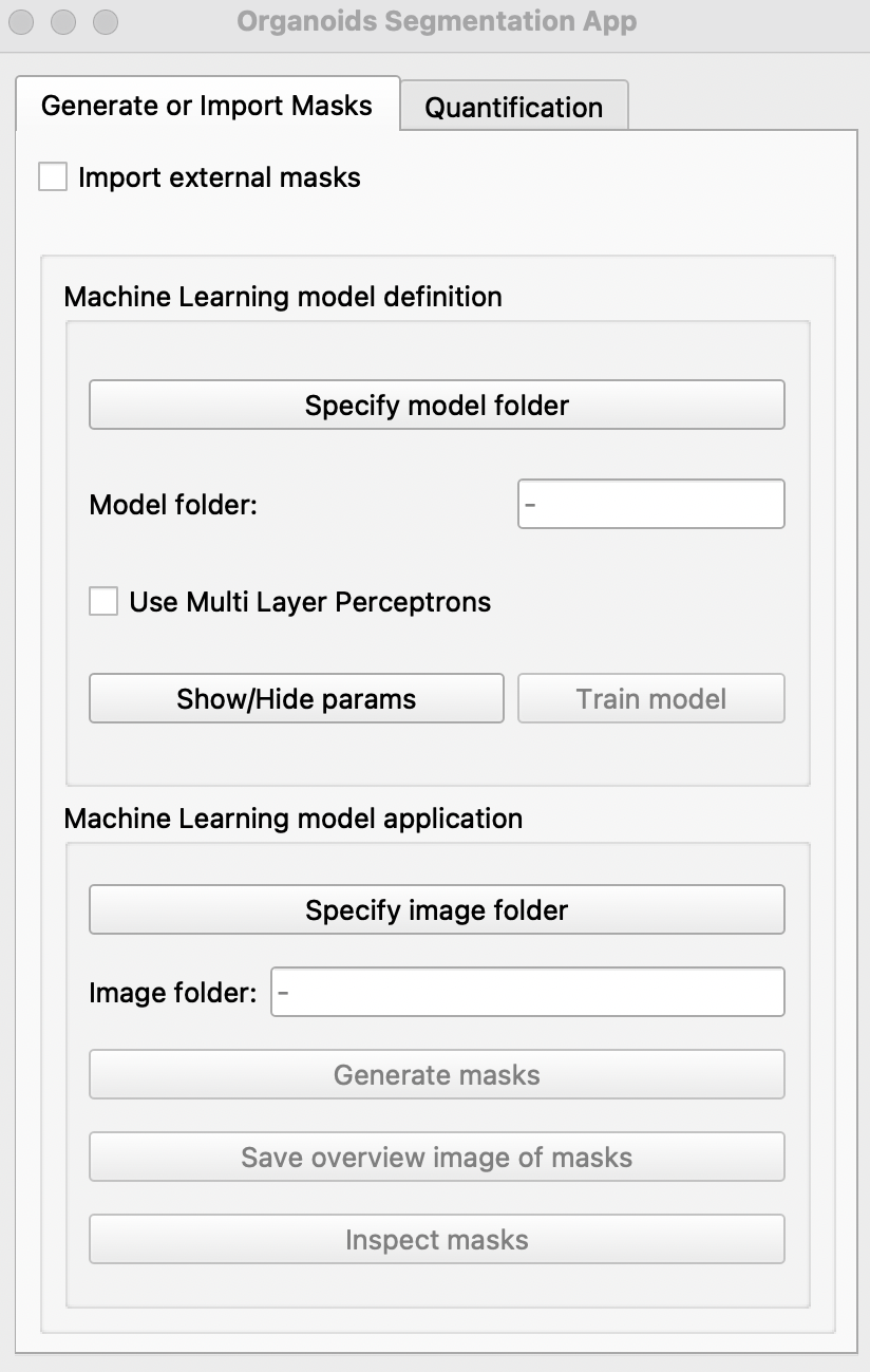
modelfolder that contains atrainingsetsub-folder. Select a few representative images (~5% of all images) and copy them into this sub-folder. If binary masks of this training set have already been created, place them in the same folder and name them as..._GT.tif. E.g.20190509_01B_dmso.tifand20190509_01B_dmso_GT.tif. -
Run the segmentation app. Click
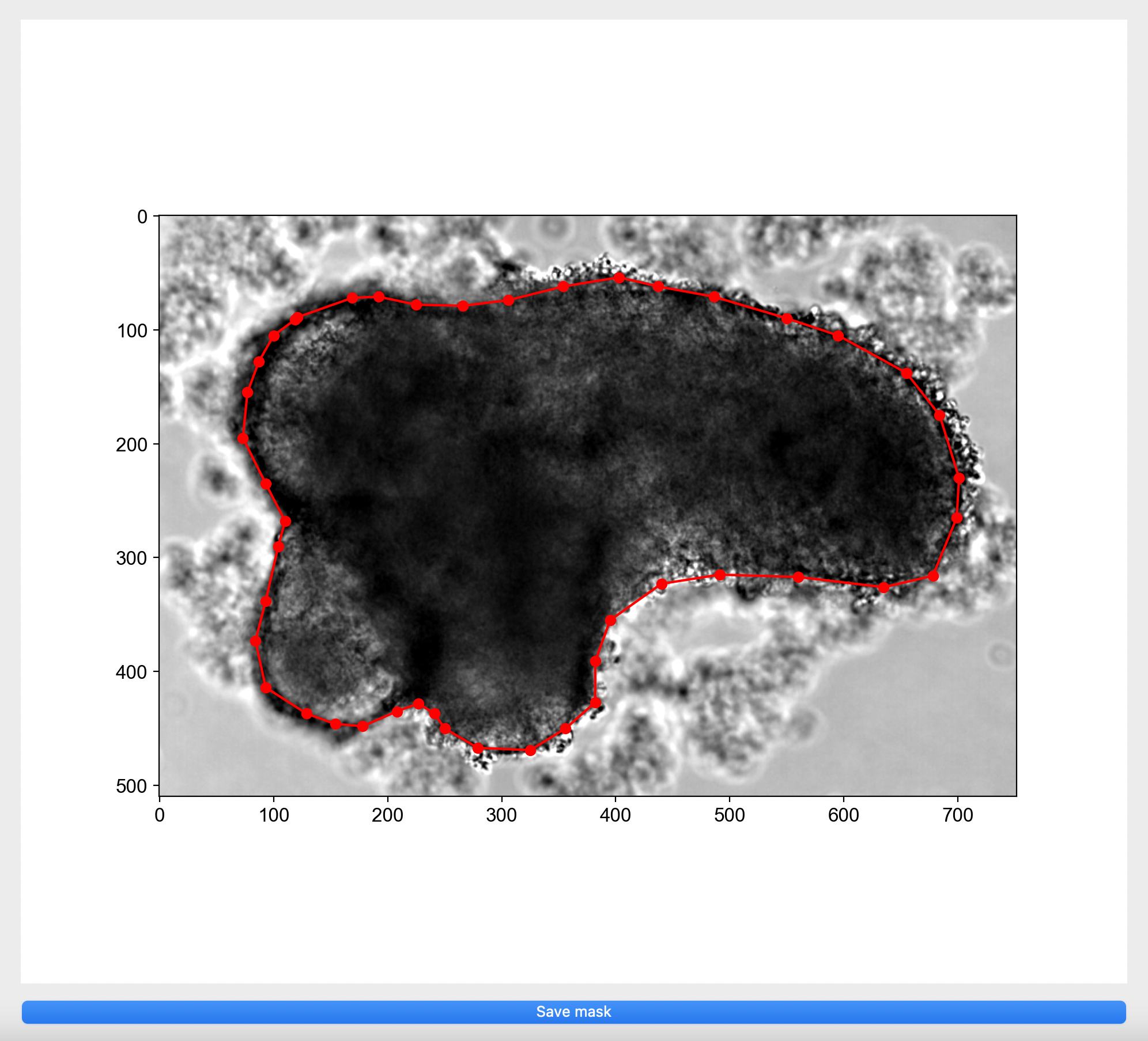
Specify model folderand select themodelfolder created. If binary masks are missing, please manually annotate for each image by clicking on the image in the pop up window to create a boundary around your object of interest or right click on red dots to remove selection.
- Select
Use Multi Layer Perceptronsif Tensorflow and CUDA have been successfully installed and if you would like to use deep learning to generate additional binary masks.
Users can choose to adjust the following parameters of the model by clicking Show/Hide params
- Sigmas: length scales (in pixels) used to generate the gaussian blurs of the input image
- Downscaling: number of pixels used to resize the input image. This is mainly done to reduce computation time, and a value of 500 is found to be enough in most applications.
- Edge size: number of pixels used on the border of the mask to generate the edge of the organoid.
- Pixel% extraction: percentage of pixels of the input image to be considered. 0: no pixels, 1: all pixels
- Extraction bias: percentage of pixels extracted from the bright region of the mask. This parameter is useful when inputted gastruloids are particularly small and there is a huge bias in extracting background pixels.
- Features: 'ilastik' or 'daisy'. In addition to the ilastik features (gaussian blur, laplacian of gaussian, difference of gaussian and gradient), daisy will compute many texture features from the inptu image. This gives more features to train on, but will slow down the training and prediction of new masks.
-
Once done, hit the
Train modelbutton. This may take some time :coffee:. Once completed, the message##### Model saved!will be seen on the terminal(MacOS) or command prompt(windows). If a model has previously been generated, select the model folder and the user can skip step 3 & 4 and jump to step 5. For models trained with Multi Layer Perceptrons, tick the option before selection of model folder. -
To generate binary masks of new images, select the folder containing images in
Specify image folderand clickGenerate masks. Once completed, the messageAll images done!will be displayed on the terminal(MacOS) or command prompt(windows). If you would like an overview of all masks generated, click onSave overview image of masksand save the pop-up image. -
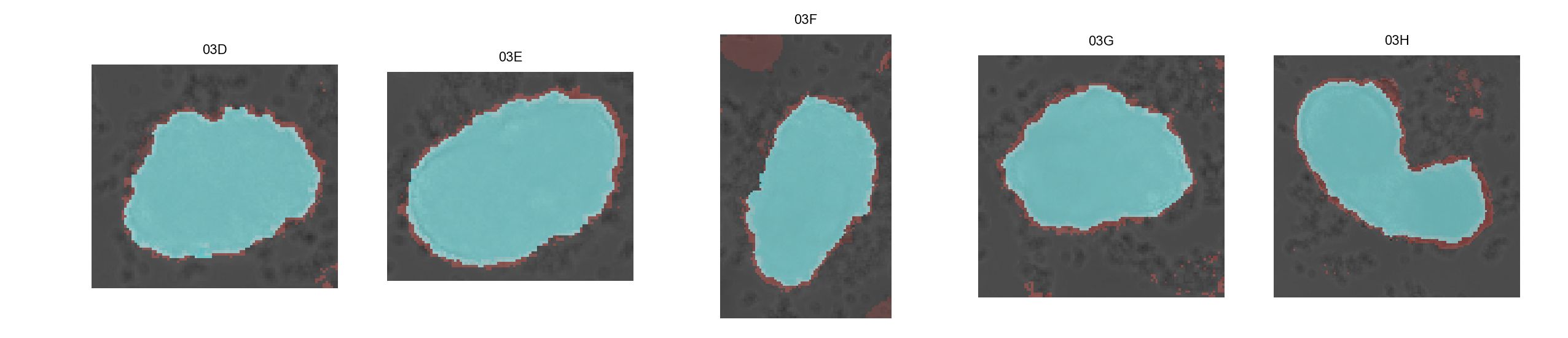
Click on
Inspect masks. This will generate a overview of binary masks overlayed with their respective brightfield images. The mask generated with the watershed algorithm is shown in blue while the red mask is generated with the classifier algorithm.
-
The other panel will allow the user to chose, for every image, the final mask type: 'ignore' (do not include selected image and mask), 'classifier' (red), 'watershed' (blue), 'manual' (manually create mask). Clicking
Show/Hide more parameterswill enable the user to change parameters such as downsampling, thinning and smoothing used in the generation of the final mask. Optional: selectCompute full meshgridto generate a meshgrid for straightening of organoid for later quantification. If disabled, meshgrid will automatically be generated later if required. -
Next,
Compute all maskswill generate the final masks for every input image and save them into theresult_segmentationsubfolder. If 'manual' is selected, the user will be prompted to generate the manual mask on a separate window. As a rule of thumb, the classifier algorithm works most of the times.
Import external masks
- If binary masks of all images have already been generated, select
Import external masks. This will reveal a new page. This feature allows import of images with multiple objects of interest.
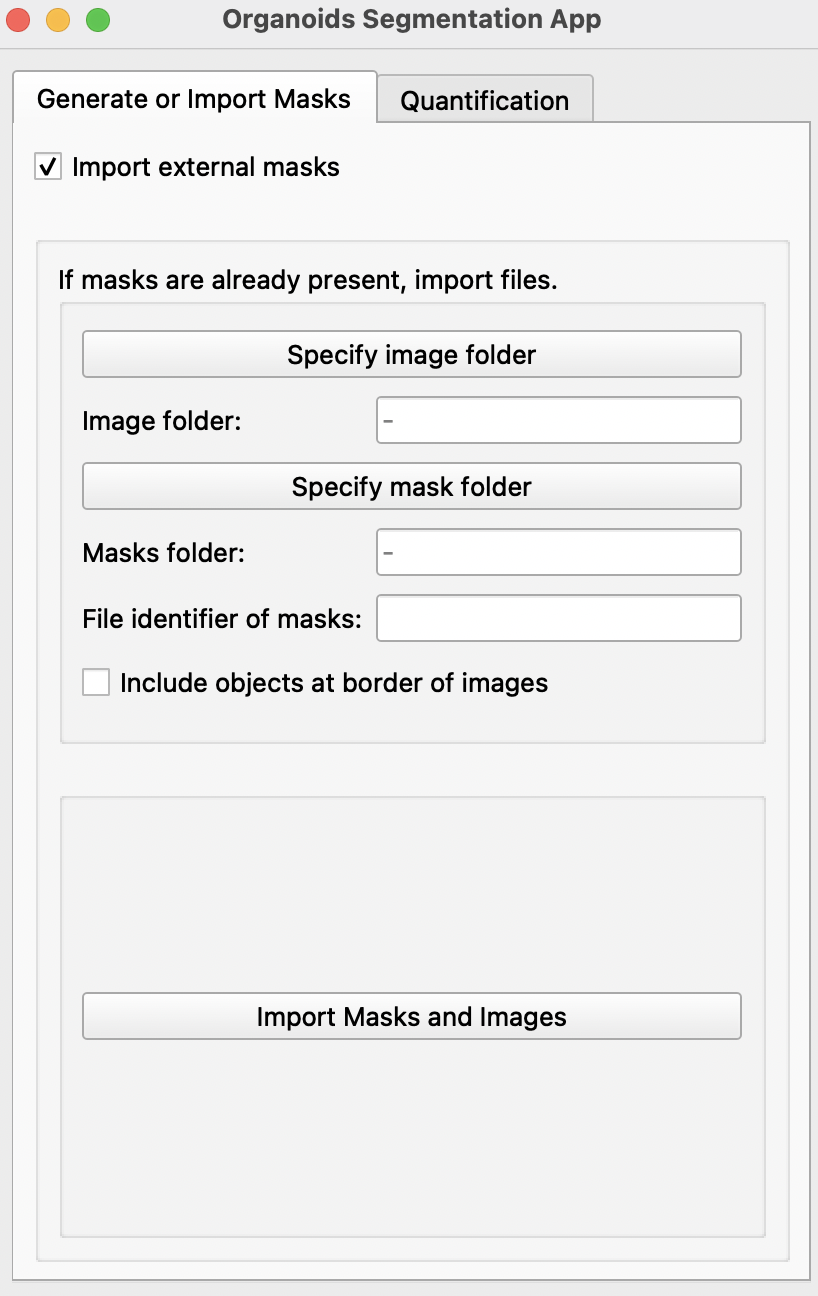
-
Specify image and mask folder with the
Specify image folderandSpecify mask folderbuttons. Masks should be labeled as name of its respective image + file identifier. E.g. if the identifier is_GT: Image20190509_01B_dmso.tifand its mask20190509_01B_dmso_GT.tif. Please ensure that masks and images are in different folders. -
Select
Include objects at border of imagesif all partial images at edges of images are to be included. -
Import Masks and Imageswill create a mask and a image for each object detected in imported images and masks.
B) Quantification
Click on the Quantification tab to enable morphological and fluorescence quantification with previously generated masks.
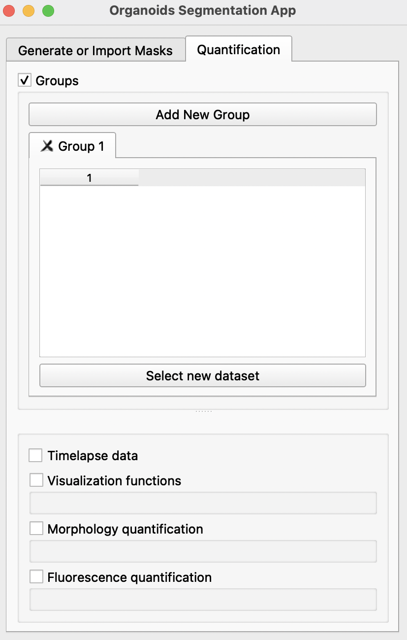
-
Using the
Select new datasetbutton, import all image folders previously generated or imported in theGenerate or Import Maskstab into the preferred groups. Each group can refer to one condition or one timepoint. For groups spanning multiple timepoints, users may select theTimelapse dataoption. More groups can be created by clickingAdd New Groupat the top. If there is only one group,Groupscan be disabled at the top after selection of dataset. -
After importing all selected image folders, there are several options available below:
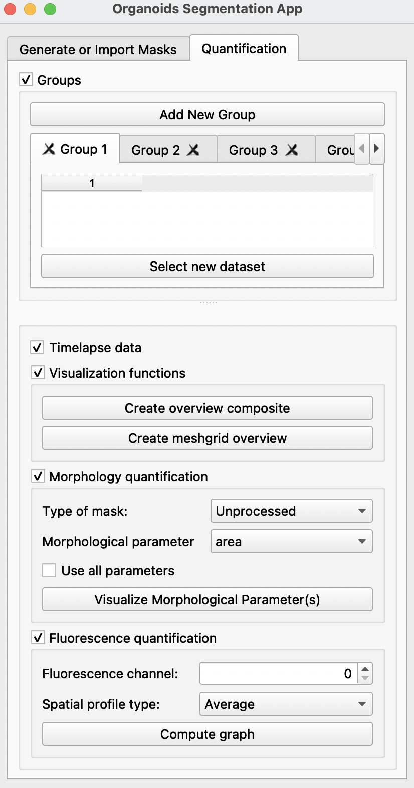
-
Visualization quantification: creates an overview of all meshgrids and composite images -
Morphology quantification: Analysis of the following morphological parameters calculated using the unprocessed mask (without straightening) or the straighted mask (straighted using the generated midline). For more information on parameters, refer to scikit-image or Sánchez-Corrales, Y. E. et al. (2018).- area
- eccentricity: ratio of the focal distance over the major axis length; value of 0 as shape approaches a circle.
- major_axis_length
- minor_axis_length
- equivalent_diameter: diameter of a circle with the same area as the region.
- perimeter
- euler_number
- extent
- orientation
- locoefa_coeff (indication of complexity of shape; refer to Sánchez-Corrales, Y. E. et al. (2018))
Use all parameters: will display 10 graphs, each a quantification of the above parameters.
Clicking
Visualize Morphological Parameter (s)will display one or more of the following windows:
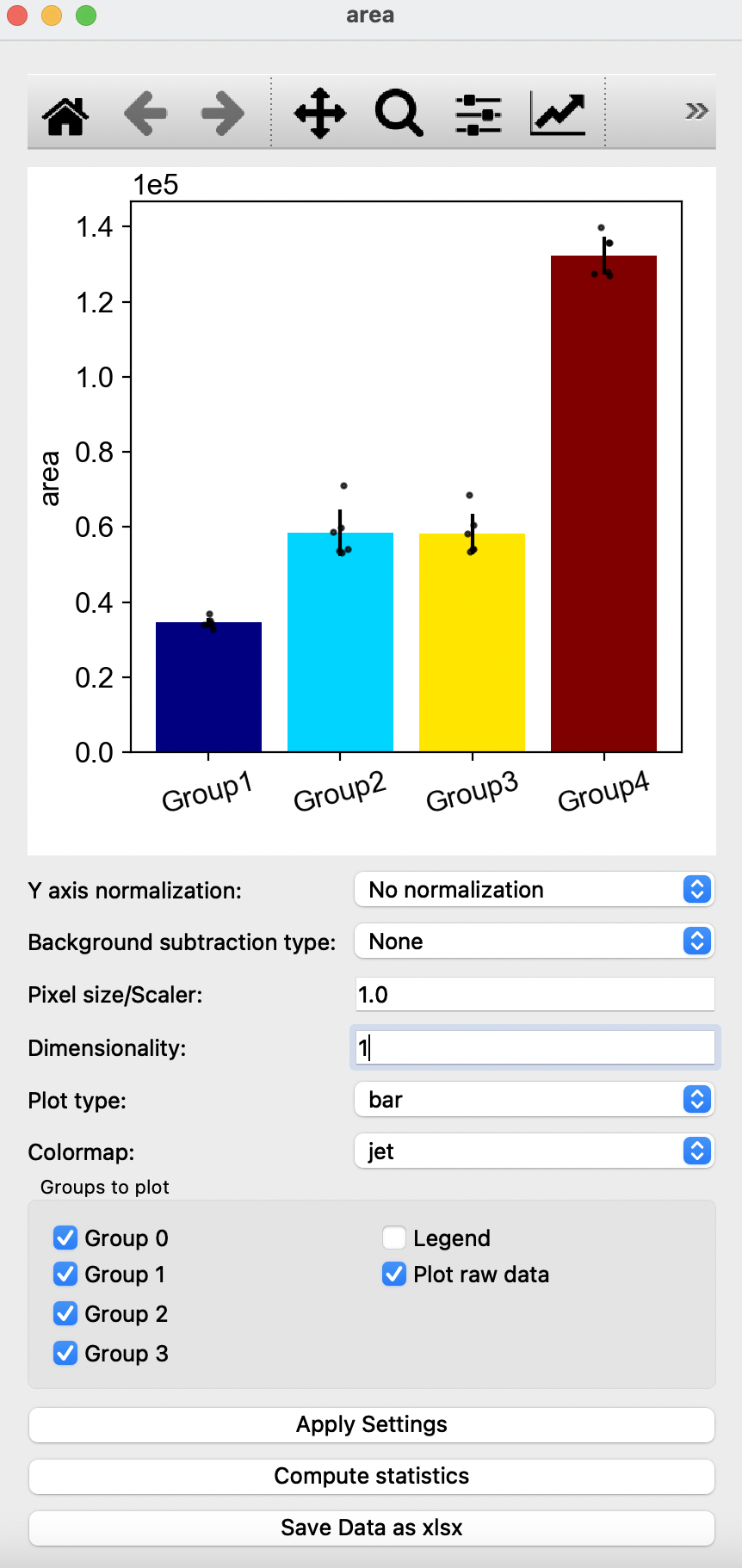
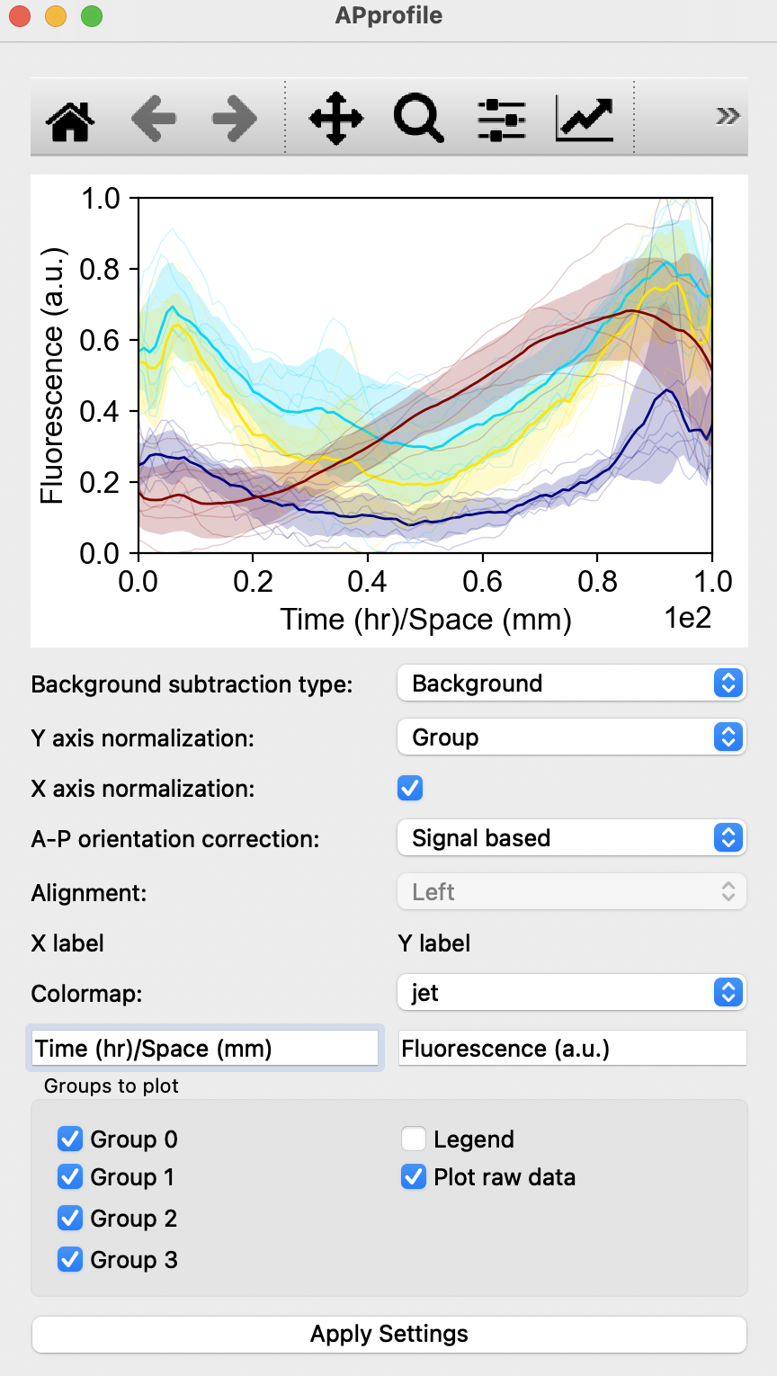
In this window, you can edit the quantification of morphological parameters by selecting the type of normalization and background subtraction. Users can also edit the graph shown by changing Pixel size/Scaler, Dimensionality, Plot type and Colormap with the options of removing groups, addition of legend or removal or raw data points on the graph. To view changes, click on Apply Settings after making the desired changes to options shown. Compute statistics shows P-values obtained from T-test, with the option of saving the p-values in a excel sheet. Users can also choose to save all resulting quantification values with the Save Data as xlsx button at the bottom. Square buttons at the top of the window can also be used to adjust the resulting graph with default options provided by matplotlib.
Fluorescence quantification: Quantification of fluorescence in the chosen channel with respect to space with the selection of Antero-Posterior profile, Left-Right profile, Radial profile, Angular profile or simply with the average fluorescence intensity.Compute graphwill display one such panel shown below:
Supplementary information
Each subfolder containing the final masks also contains a segmentation_params.csv file generated during mask generation with the following information selected during creation of binary masks:
- filename
- chosen_mask: classifier (c), watershed (w), manual (m), ignore (i)
- down_shape
- thinning
- smoothing
All morphological properties of organoids are computed when required and saved as ..._morpho_params.json into the same subfolder as the final masks (result_segmentation)
These include:
- 'input_file'
- 'mask_file'
- 'centroid'
- 'slice'
- 'area'
- 'eccentricity' (perfect circle:0, elongated ellipse:~1)
- 'major_axis_length'
- 'minor_axis_length'
- 'equivalent_diameter'
- 'perimeter'
- 'anchor_points_midline'
- 'N_points_midline'
- 'x_tup'
- 'y_tup'
- 'midline'
- 'tangent'
- 'meshgrid_width'
- 'meshgrid'
The _morpho_straight_params.json is computed when required and saved into the same subfolder as the final masks (result_segmentation). It contains the following infomation:
- area
- eccentricity
- major_axis_length
- minor_axis_length
- equivalent_diameter
- perimeter
- euler_number
- extent
- orientation
- locoefa_coeff (indication of complexity of shape)
The average fluorescence intensities, and those along the Antero-Posterior, Left-Right, Radial and Angular profile of organoids are computed when required and saved as ..._fluo_intensity.json into the same subfolder as the final masks (result_segmentation).
Release history Release notifications | RSS feed


Download files
Download the file for your platform. If you're not sure which to choose, learn more about installing packages.
Source Distribution
Built Distribution
Filter files by name, interpreter, ABI, and platform.
If you're not sure about the file name format, learn more about wheel file names.
Copy a direct link to the current filters
File details
Details for the file morgana-0.1.1.tar.gz.
File metadata
- Download URL: morgana-0.1.1.tar.gz
- Upload date:
- Size: 8.5 MB
- Tags: Source
- Uploaded using Trusted Publishing? No
- Uploaded via: twine/3.4.1 importlib_metadata/3.10.0 pkginfo/1.6.1 requests/2.24.0 requests-toolbelt/0.9.1 tqdm/4.61.0 CPython/3.8.5
File hashes
| Algorithm | Hash digest | |
|---|---|---|
| SHA256 |
f7839dc28eda53c90d4ffd6d0c79231acebbe6a525f503f0ef1fb3c05e228cdd
|
|
| MD5 |
96b435c845503c1f2fc463dc9dbefca6
|
|
| BLAKE2b-256 |
2b91160439aee268f8d9312ed3e725e5dd29ff881b1901c98c9430fee00069c3
|
File details
Details for the file morgana-0.1.1-py3-none-any.whl.
File metadata
- Download URL: morgana-0.1.1-py3-none-any.whl
- Upload date:
- Size: 8.7 MB
- Tags: Python 3
- Uploaded using Trusted Publishing? No
- Uploaded via: twine/3.4.1 importlib_metadata/3.10.0 pkginfo/1.6.1 requests/2.24.0 requests-toolbelt/0.9.1 tqdm/4.61.0 CPython/3.8.5
File hashes
| Algorithm | Hash digest | |
|---|---|---|
| SHA256 |
492900f329072ac5130f676d29e87faff3b7b2fa66d97e0033048d959404193a
|
|
| MD5 |
e3de66b5b8e827d251c247440cff6059
|
|
| BLAKE2b-256 |
52f4b55c4b6318f43e1b02738cfd2f452c2f661ab86c8b1fb873b51ba8eecd57
|


