A Python plotting library for visualization of basketball data.


Project description

A Python plotting library to visualize basketball data, created by the Sport Performance Lab (SPL) at Maple Leaf Sports & Entertainment (MLSE), Toronto, Canada.
Sport Performance Lab (SPL) is a Research and Development group that works across all MLSE teams on strategic research initiatives in sports analytics and player performance.
Quick start
Install the package using pip (or pip3).
pip install mplbasketball
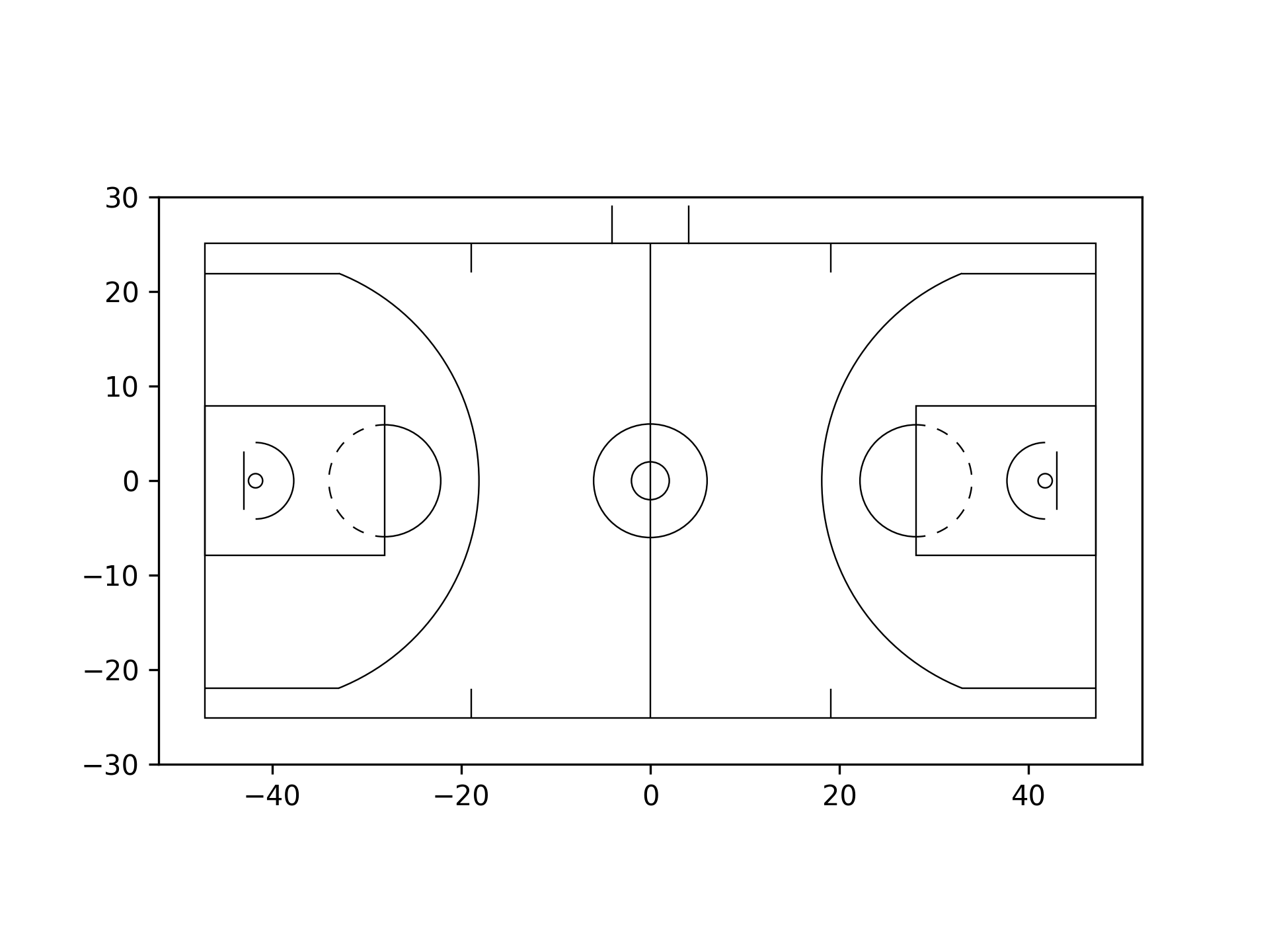
Plot an NBA basketball court, with the origin at center court, and measuring in feet (currently "ft" and "m" are supported):
from mplbasketball import Court

court = Court(court_type="nba", origin="center", units="ft")
fig, ax = court.draw(showaxis=True)
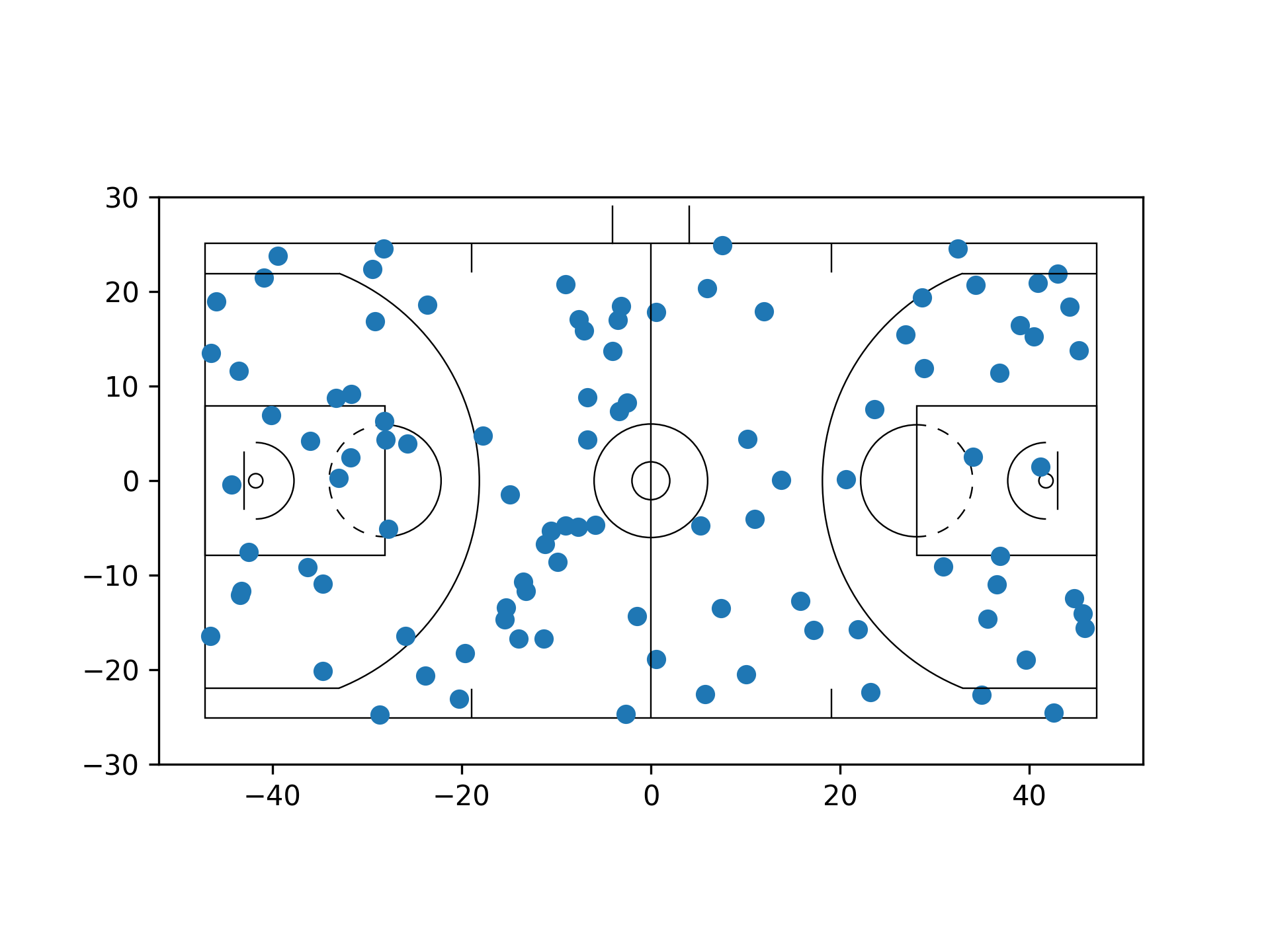
Plot some points on the court:
import numpy as np

n_points = 100
x = np.random.uniform(-47, 47, size=n_points)
y = np.random.uniform(-25, 25, size=n_points)

ax.scatter(x, y)
List of capabilities
Currently, you can use mplbasketball to
- Plot 2D and 3D spatio-temporal basketball data from 3 major basketball competitions
- View data in different orientations orientation (horizontal, vertical, and also normalized to left/right/up/down). The
utils.transformfunction makes going between orientations extremely easy and seamless. - Easily interface with existing
matplotlibfunctions.
Before you begin
Some notes on plotting data using mplbasketball:
- Ensure your 2D data is in a right-handed coordinate system (RHCS). Many data providers (including the NBA) provide their data using left handed coordinate systems (LHCS). If you obtain data in an LHCS, simply flip the sign of all the
ycomponents (assuming data is left-right), making it compatible with plotting usingmplbasketball.
Usage
The Court class
The Court class comprises of the dimensions of the basketball court under consideration. When being defined, it takes in a court_type, which can currently be "nba" (default), "wnba", or "ncaa". Court dimension measurements are provided in mplbasketball/court_params.py. The Court class has a method draw(), which will draw the court in any desired orientation:
"h": horizontal (default)"v": vertical"hl": horizontal, only left side"hr": horizontal, only right side"vu": vertical, only up side"vd": vertical, only down side
The draw() method can either be called to define a matplotlib fig and ax object using:
from mplbasketball import Court

court = Court(origin="top-left")
fig, ax = court.draw(orientation="h")
After this, you can simply plot your data on the ax object. Note that you may need to adjust the zorder to ensure all elements are properly visible.
Setting the origin
The package allows for the origin of the data to be in 5 locations on the court (numbers quoted below are in feet, and in accordance with the NBA handbook's court dimensions, when using "m" as the unit, simply multiply the numbers below by the appropriate conversion factor):
"center": Center court and the origin coincide."top-left": Center court is at[47, -25]."bottom-left": Center court is at[47, 25]."top-right": Center court is at[-47, -25]."bottom-right": Center court is at[-47, 25].
The origin should be specified in the initial specification of the Court object. To see what the x and y ranges are for each origin choice, see this document. These origin conventions assume the data is in the left-right direction.
Transforming data to different orientations
Often, it is more useful to view data from different perspectives. As mentioned in the preceding section, there are 6 orientations to view 2D spatiotemporal data in mplbasketball. The utils.transform() function makes it very easy to change perspective. We first load some data in its original form; say we are working with a dataset that uses the "bottom-left" part of the court as the origin.
import numpy as np
import matplotlib.pyplot as plt
from mplbasketball import Court
from mplbasketball.utils import transform

# Initialize Court object
origin = "bottom-left"
court = Court(origin=origin)
fig, ax = plt.subplots(1, 3)

# Simulate some data
n_pts = 100
x_1 = np.random.uniform(0, 94, size=n_pts)
y_1 = np.random.uniform(0, 50, size=n_pts)

x_2 = np.random.uniform(0, 94, size=n_pts)
y_2 = np.random.uniform(0, 50, size=n_pts)

# On the first subplot, plot the data as is
court.draw(ax[0], )
ax[0].scatter(x, y, s=5, c="tab:blue")
ax[0].scatter(x, y, s=5, c="tab:orange")
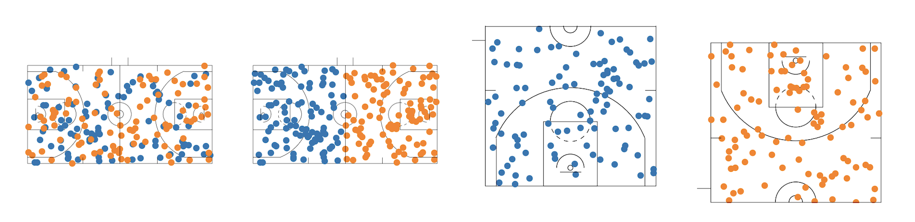
Now, say we want to visualize the first (blue) dataset normalized to the left side, and the second (orange) dataset normalized to the right. In the second subplot, we can transform the data such that all of the points are normalized to their respective side.
x_1_hl, y_1_hl = transform(x_1, y_1, fr="h", to="hl", origin=origin)
x_2_hr, y_2_hr = transform(x_2, y_2, fr="h", to="hr", origin=origin)
court.draw(ax[1], )
ax[1].scatter(x_1_hl, y_1_hl, s=5, c="tab:blue")
ax[1].scatter(x_2_hr, y_2_hr, s=5, c="tab:orange")
Here, the fr and to arguments tell the function what orientation the data currently is in, and what the desired orientation is, respectively. Finally, we can visualize this left-normalized data on a vertical court. Say we want to look at the blue data with the hoop at the bottom (the "vd" orientation), and the orange data with the hoop at the top. This is again very easy:
x_1_vd, y_1_vd = transform(x_1_hl, y_1_hl, fr="hl", to="vd", origin=origin)
court.draw(ax[2], orientation="vd")
ax[2].scatter(x_1_vd, y_1_vd, s=5, c="tab:blue")

x_2_vu, y_2_vu = transform(x_2_hr, y_2_hr, fr="hl", to="vu", origin=origin)
court.draw(ax[3], orientation="vu")
ax[3].scatter(x_2_vu, y_2_vu, s=5, c="tab:orange")
The final result looks like this:
Some notes about the above:
- To produce data for the final plot, we could have also used
x_1_vd, y_1_vd = transform(x_1, y_1, fr="h", to="vd", origin=origin)
- To show more/less of the court markings, we can make use of the
zorderargument in theax.scatterplots.
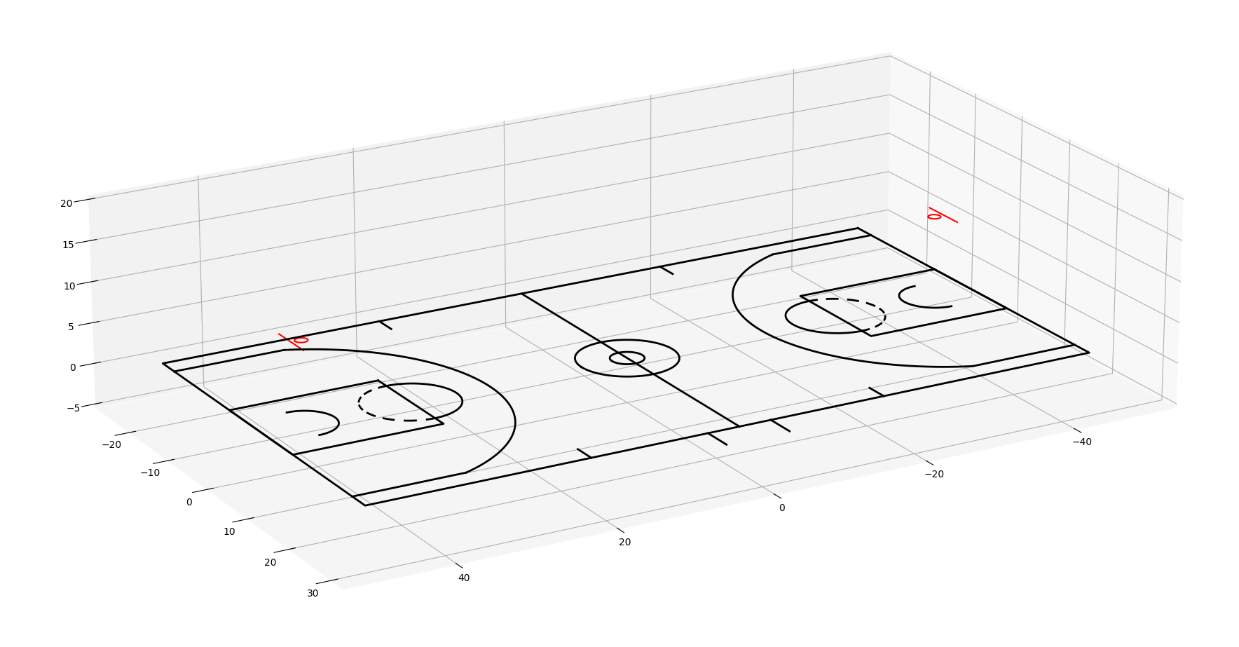
3D Court plotting
The court3d module allows for the plotting of 3D basketball data, particularly useful when visualizing 3D ball motion, or in cases where body pose data is available. The draw_court_3d() function is the quickest way to obtain a drawing of a court in 3D space.
from mplbasketball.court3d import draw_court_3d
import matplotlib.pyplot as plt

zlim = 20

fig = plt.figure(figsize=(20, 20))
ax = fig.add_subplot(111, projection="3d")
# Set up initial plot properties
ax.set_zlim([0, zlim])

draw_court_3d(ax, origin=np.array([0.0, 0.0]), line_width=2)
Interfacing with matplotlib functions
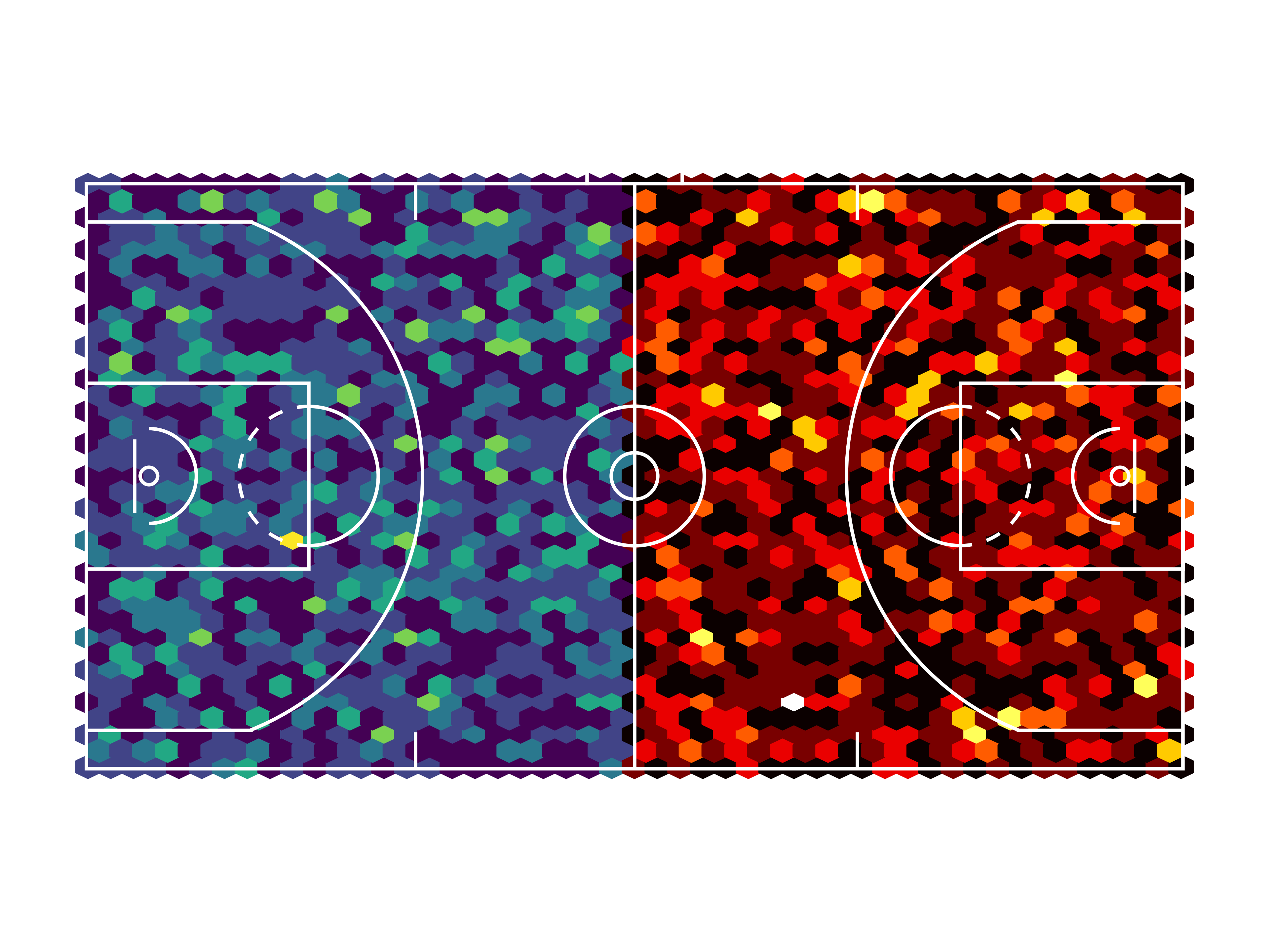
Hex-binning
import numpy as np
import matplotlib.pyplot as plt
from mplbasketball import Court
from mplbasketball.utils import transform

# Initialize Court object
origin = "bottom-left"
court = Court(origin=origin)
fig, ax = plt.subplots()

# Simulate some data
n_pts = 1000
x_1 = np.random.uniform(0, 94, size=n_pts)
y_1 = np.random.uniform(0, 50, size=n_pts)
x_2 = np.random.uniform(0, 94, size=n_pts)
y_2 = np.random.uniform(0, 50, size=n_pts)

# Transform the data
x_1_hl, y_1_hl = transform(x_1, y_1, fr="h", to="hl", origin=origin)
x_2_hr, y_2_hr = transform(x_2, y_2, fr="h", to="hr", origin=origin)

# Draw the court, slightly thicken the lines
court.draw(ax, line_color="white", line_width=0.3)

# Hex-bin the data, while ensuring that the court is plotted on top
ax.hexbin(x_1_hl, y_1_hl, gridsize=(24, 18), extent=(0, 47, 0, 50), zorder=0)
ax.hexbin(x_2_hr, y_2_hr, gridsize=(24, 18), extent=(47, 94, 0, 50), zorder=0 , cmap="hot")
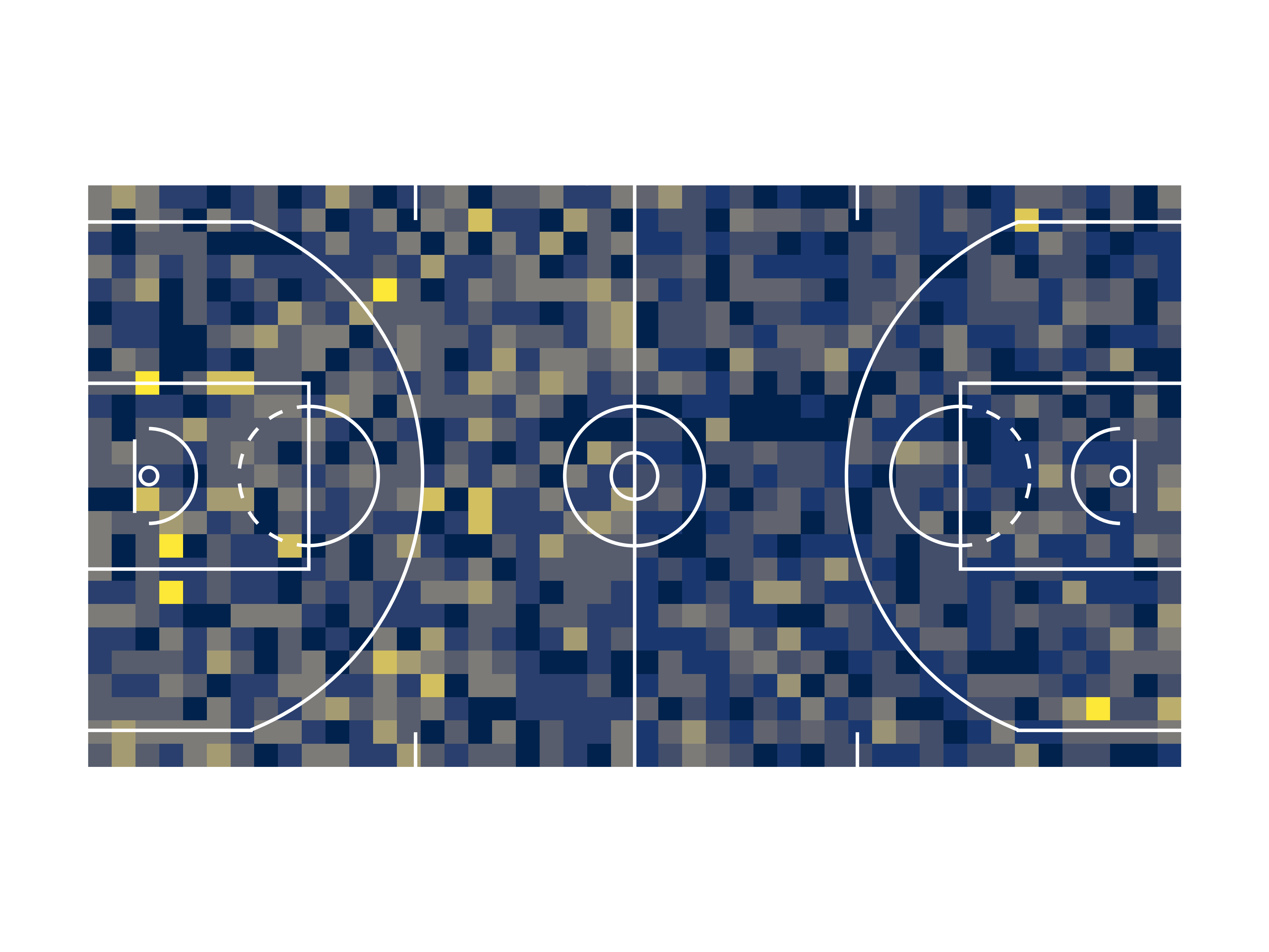
Heatmaps
# Compute the heatmap
heatmap_1, xedges_1, yedges_1 = np.histogram2d(x_1, y_1, bins=(94//4, 50//2), range=[[0, 94/2], [0, 50]])
heatmap_2, xedges_2, yedges_2 = np.histogram2d(x_2, y_2, bins=(94//4, 50//2), range=[[94/2, 94], [0, 50]])

# Draw the court, slightly thicken the lines
fig, ax = court.draw(line_color="white", line_width=0.3)

# Display the heatmaps
extent_1 = [xedges_1[0], xedges_1[-1], yedges_1[0], yedges_1[-1]]
extent_2 = [xedges_2[0], xedges_2[-1], yedges_2[0], yedges_2[-1]]

ax.imshow(heatmap_1.T, extent=extent_1, origin='lower', cmap='cividis', zorder=-1)
ax.imshow(heatmap_2.T, extent=extent_2, origin='lower', cmap='cividis', zorder=-1)
Documentation
Full documentation coming soon. In the meantime, check out the examples in this README, as well as some of our examples!
Contribute
We welcome feedback and contributions to this package - browse the open issues, or open a pull request!
Inspirations
This package is takes inspiration from mplsoccer, one of the first and best-written sports plotting libraries. Many of the structural decisions made here have been inspired by mplsoccer's Pitch class.
License
Release history Release notifications | RSS feed


Download files
Download the file for your platform. If you're not sure which to choose, learn more about installing packages.
Source Distribution
Built Distribution
Filter files by name, interpreter, ABI, and platform.
If you're not sure about the file name format, learn more about wheel file names.
Copy a direct link to the current filters
File details
Details for the file mplbasketball-1.0.0.tar.gz.
File metadata
- Download URL: mplbasketball-1.0.0.tar.gz
- Upload date:
- Size: 17.7 kB
- Tags: Source
- Uploaded using Trusted Publishing? No
- Uploaded via: twine/5.1.1 CPython/3.12.3
File hashes
| Algorithm | Hash digest | |
|---|---|---|
| SHA256 |
efeb41f9d6d32989b6bdfe2b66c131e4797f621e8820c6e842a0f071d1d2106e
|
|
| MD5 |
56ddb90a2ad920c3a66c522763fc8273
|
|
| BLAKE2b-256 |
9e4b210622de52166f2028d9c0593de7abc1ac4a8d995ab1e8da4b7d519e8b83
|
File details
Details for the file mplbasketball-1.0.0-py3-none-any.whl.
File metadata
- Download URL: mplbasketball-1.0.0-py3-none-any.whl
- Upload date:
- Size: 16.5 kB
- Tags: Python 3
- Uploaded using Trusted Publishing? No
- Uploaded via: twine/5.1.1 CPython/3.12.3
File hashes
| Algorithm | Hash digest | |
|---|---|---|
| SHA256 |
397dc30b583ad2799325354bfd8bd9d8a6f5b6375d45172a952c4d9961bcc4a5
|
|
| MD5 |
bd7cea76b2fb3949839f27ea3f0b411f
|
|
| BLAKE2b-256 |
3932d00f52eb0810c59cb5a31b69140685ff9983bd9b83ee12bd97ab51385d23
|


