A Python port of R package mshap to interpret combined model outputs.

Project description
mshap

This is a Python port of srmatth/mshap
The goal of mshap is to allow SHAP values for two-part models to be easily computed. A two-part model is one where the output from one model is multiplied by the output from another model. These are often used in the Actuarial industry, but have other use cases as well.
Installation
Install mSHAP from pypi with the following code:
pip install mshap
Or the development version from github with:
pip install git+https://github.com/Diadochokinetic/mshap
Basic Use
We will demonstrate a simple use case on simulated data. Suppose that we wish to be able to predict to total amount of money a consumer will spend on a subscription to a software product. We might simulate 4 explanatory variables that looks like the following:
import numpy as np

age = np.random.uniform(18, 60, size=1000)
income = np.random.uniform(50000, 150000, size=1000)
married = np.random.randint(0, 2, size=1000)
sex = np.random.randint(0, 2, size=1000)
Now because this is a contrived example, we will knowingly set the
response variables as follows (suppose here that cost_per_month is
usage based, so as to be continuous):
cost_per_month = (0.0006 * income - 0.2 * sex + 0.5 * married - 0.001 * age) + 10
num_months = 15 * (0.001 * income * 0.001 * sex * 0.5 * married - 0.05 * age) ** 2
Thus, we have our data. We will combine the covariates and target variables into a single data frame for ease of use in python.
import pandas as pd

data = pd.DataFrame(
    {
        "age": age,
        "income": income,
        "married": married,
        "sex": sex,
        "cost_per_month": cost_per_month,
        "num_months": num_months,
    }
)
The end goal of this exercise is to predict the total revenue from the given customer, which mathematically will be cost_per_month * num_months. Instead of multiplying these two vectors together initially, we will instead create two models: one to predict cost_per_month and the other to predict num_months. We can then multiply the output of the two models together to get our predictions.
We now create our two models and predict on the training sets:
from sklearn.ensemble import RandomForestRegressor

X = data[["age", "income", "married", "sex"]]
y1 = data["cost_per_month"]
y2 = data["num_months"]

cpm_mod = RandomForestRegressor(n_estimators=100, max_depth=10, max_features=2)
cpm_mod.fit(X, y1)
# > RandomForestRegressor(max_depth=10, max_features=2)
nm_mod = RandomForestRegressor(n_estimators=100, max_depth=10, max_features=2)
nm_mod.fit(X, y2)
# > RandomForestRegressor(max_depth=10, max_features=2)
cpm_preds = cpm_mod.predict(X)
nm_preds = nm_mod.predict(X)

tot_rev = cpm_preds * nm_preds
We will now proceed to use TreeSHAP and subsequently mSHAP to explain the ultimate model predictions.
import shap

cpm_ex = shap.Explainer(cpm_mod)
cpm_shap = cpm_ex.shap_values(X)
cpm_expected_value = cpm_ex.expected_value

nm_ex = shap.Explainer(nm_mod)
nm_shap = nm_ex.shap_values(X)
nm_expected_value = nm_ex.expected_value
from mshap import Mshap

final_shap = Mshap(
    cpm_shap, nm_shap, cpm_expected_value, nm_expected_value
).shap_values()
final_shap
{'shap_vals':                0            1          2          3
 0   -2876.216193   325.130506  13.474704 -26.475439
 1    1950.301864   200.312921 -11.558773 -64.926704
 2   -2092.259421  -734.279715   7.840975  15.369813
 3    2735.235840 -1642.421894 -11.395891 -63.590990
 4    1971.574419  -878.331239 -20.712473  36.722350
 ..           ...          ...        ...        ...
 995 -1261.220638  1439.860900   2.017464  48.838624
 996  1291.397944  -553.954467 -27.043572 -50.365440
 997  1320.930428  -492.378408 -20.519565 -50.760569
 998  1156.518243  -415.144837  20.484928  59.726275
 999 -3375.016633   732.381880 -33.174228 -86.247622

 [1000 rows x 4 columns],
 'expected_value': 4284.231240147299}
You can put the result into a shap Explanation object to use shap plot capabilities:
final_shap_explanation = shap.Explanation(
    values=final_shap["shap_vals"].values,
    base_values=final_shap["expected_value"],
    data=X,
    feature_names=X.columns,
)
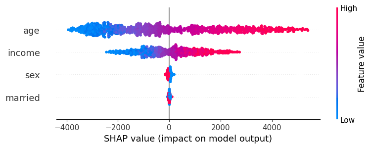
shap.summary_plot(final_shap_explanation, X)
Citations
- For more information about SHAP values in general, you can visit theSHAP github page
- If you use
{mshap}, please cite mSHAP: SHAP Values for Two-Part Models


Download files
Download the file for your platform. If you're not sure which to choose, learn more about installing packages.
Source Distribution
Built Distribution
Filter files by name, interpreter, ABI, and platform.
If you're not sure about the file name format, learn more about wheel file names.
Copy a direct link to the current filters
File details
Details for the file mshap-0.2.3.tar.gz.
File metadata
- Download URL: mshap-0.2.3.tar.gz
- Upload date:
- Size: 59.5 kB
- Tags: Source
- Uploaded using Trusted Publishing? No
- Uploaded via: twine/6.2.0 CPython/3.9.25
File hashes
| Algorithm | Hash digest | |
|---|---|---|
| SHA256 |
3ca748d612bd5e98b4b2e148bd4dd36da239dc91eda79769151a0e49428ab54d
|
|
| MD5 |
b871087c0cfcd0ea52fc209bd3712c87
|
|
| BLAKE2b-256 |
1ef788e875f702ce3ff9e942975d315c3ca60d84657a57b81965c7b656adf806
|
File details
Details for the file mshap-0.2.3-py3-none-any.whl.
File metadata
- Download URL: mshap-0.2.3-py3-none-any.whl
- Upload date:
- Size: 8.7 kB
- Tags: Python 3
- Uploaded using Trusted Publishing? No
- Uploaded via: twine/6.2.0 CPython/3.9.25
File hashes
| Algorithm | Hash digest | |
|---|---|---|
| SHA256 |
1fe8c67962cb2027896d1b882fbc13f191f589d3c436bc8d28199778a8674d3e
|
|
| MD5 |
1c61ab9a5afcdbdb32bfcb0a0c951d6a
|
|
| BLAKE2b-256 |
84e5ebe543ae7b181086f1b087fba3c785e34c2703069501e5b6fb95e30c1ff6
|


