
Nano_ext: Nanopore Signal Event Extraction
A Python toolkit (with Rust extensions) for extracting ionic-current blockade events from high-sampling-rate (>100 kHz) nanopore traces. Nano_ext uses objective, information-criterion-based and Bayesian methods throughout — no manual threshold tuning required — and handles 10-minute, 250 kHz recordings on a laptop.
pip install "nano-ext[gui]"
nano-ext gui            # opens the analysis app in your browser
Screenshots
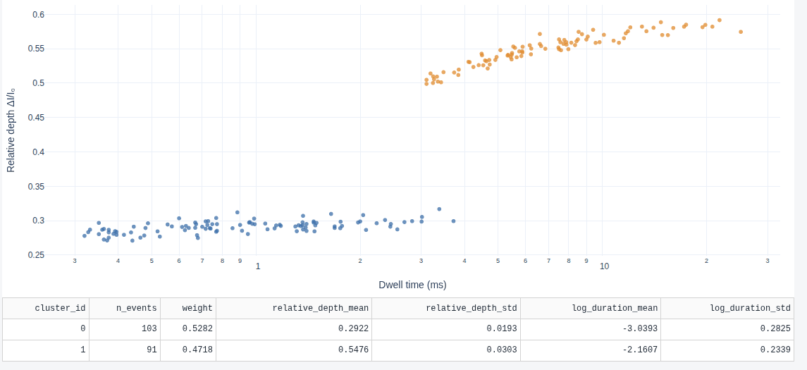
Browser GUI — event populations
Interactive Jupyter UI

Waveform Analysis

Features
- Browser GUI (
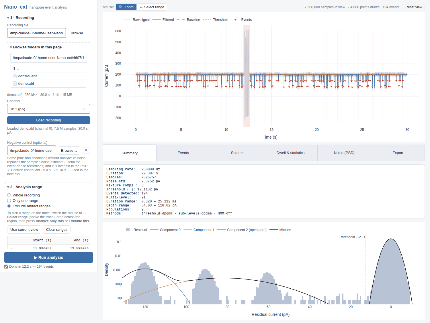
nano-ext gui): load ABF / raw binary files, zoom smoothly through 150 M-sample traces (view-dependent min/max downsampling), drag or zoom to exclude artifacts, run any analysis method, and inspect events, populations, dwell-time fits and noise spectra — then export CSV / JSON. Runs locally; your data never leave the machine. - Objective Thresholding: a Dirichlet-process Gaussian mixture (default since 1.2; GMM + BIC remains available) infers the number of current levels and places the detection threshold between the open-pore and event components.
- Objective Sub-level Analysis: the same Dirichlet-process mixture, fitted on decorrelated samples within each event, identifies sub-steps without user-tuned sigma thresholds. On synthetic benchmarks it recovers the true number of levels for 100 % of events (GMM + BIC: 66 %).
- Drift Handling: Iterative local baseline estimation with polynomial/spline global detrending handles gradual open-pore current shifts.
- Multi-directional Detection: Detect downward blockades, upward deflections, or both simultaneously. Each event is tagged with its direction.
- Automated Parameter Tuning:
suggest_config()estimates the noise floor from the signal and automatically setsmin_event_duration,merge_gap, andbaseline_window— a good starting point before manual refinement. - Negative Control Integration: Pass an analyte-free control recording to derive a clean noise estimate, stabilising threshold determination when the sample trace is event-dense.
- Artifact Exclusion: Exclude one or more artifact regions (e.g. from zapping operations) from all estimation steps via
--analysis-range START END(single keep-window) or--exclude-range START END(one or more exclusion windows). Event timestamps in the output remain in original-file coordinates. - High Performance: Rust extensions (PyO3/maturin) accelerate the sliding-window baseline percentile (multi-threaded, selection instead of sorting) and PELT change-point kernels. Per-event sub-level analysis runs in parallel worker processes (
--jobs, default: all CPUs). - Long Recordings on a Laptop: ABF data are memory-mapped and kept as float32 (exact for 16-bit ADC data); time arrays are implied rather than stored. A 10-minute, 250 kHz recording (150 M samples) runs end-to-end in ~1.5 min with a ~3.3 GB peak (see Performance).
- Flexible Input: Supports Axon Binary Format (ABF) and raw binary data.
- Interactive Jupyter UI:
notebooks/interactive_analysis.ipynbprovides a widget-based GUI for interactive parameter exploration and result inspection — no terminal required during analysis. - Per-Event Waveform Viewer: Browse individual events with zoomed two-panel figures (signal + residual + sublevel boundaries). Export any event's waveform as
.npzor.csvfor downstream ML workflows. - HMM Multi-state Analysis: Gaussian HMM fitting per event with BIC-based state-count selection. Reports state means, transition matrix, and dwell-time distributions. Enable with
--hmm(requirespip install "nano_ext[hmm]"), or use--hmm-method sticky_hdpfor a sticky HDP-HMM that infers the number of states (no extra dependency). - Selectable Methods:
--threshold-method {dpgmm,gmm}and--sublevel-method {dpgmm,gmm,bocpd}(defaultdpgmm;gmmreproduces results from ≤ 1.1). Bayesian online change-point detection (bocpd) is experimental — it over-segments traces with strong 1/f noise. - Event Population Clustering:
--clustergroups events into populations (relative depth × log dwell time) with a Dirichlet-process GMM — the number of populations is inferred, and each event gets a membership probability. - Bayesian Event Statistics:
--bayes-statsreports the capture rate with a credible interval and fits a mixture of exponentials to dwell times, giving the posterior number of time constants and their credible intervals (per population with--cluster). - Power Spectral Density: Welch-method PSD for noise diagnostics and effective filter-cutoff estimation. Compare sample vs. control with
nano-ext spectrumor the Diagnostics panel in the Jupyter UI. - Comprehensive Output: Per-event CSV summaries, per-sub-level CSV (joinable via
event_id), and interactive plotly visualisations.
Installation
From PyPI
Pre-built wheels (Linux x86_64/aarch64, macOS Intel/Apple silicon, Windows x64; CPython ≥ 3.10) — no Rust toolchain needed.
pip install nano-ext            # analysis library + CLI
pip install "nano-ext[gui]"     # + browser GUI (Dash)
pip install "nano-ext[hmm]"     # + EM/BIC HMM (hmmlearn)
pip install "nano-ext[all]"     # everything, including the Jupyter UI
From Source (Development Mode)
Requires a Rust toolchain (rustup) because the package includes a compiled Rust extension.
git clone https://github.com/gorgeouspig/Nano_ext.git
cd Nano_ext
python -m venv .venv && source .venv/bin/activate   # or a conda environment
pip install -e ".[dev,gui,hmm]"   # compiles the Rust extension via maturin
pytest                            # fast tests; `pytest -m slow` for the rest
Quick Start
Browser GUI
nano-ext gui                      # start in the current folder
nano-ext gui recording.abf        # pre-select a file
nano-ext gui --port 8060 --no-browser
The app opens at http://127.0.0.1:8050/. Work top to bottom in the left panel:
- Recording — press Browse… to pick a file with your system's file dialog (or paste a path, or use Browse folders in this page); the recording loads as soon as you choose it. Pick the channel for multi-channel ABF files; raw binary files ask for the sampling rate and data type. Optionally choose a negative control (analyte-free recording): its noise replaces the sample's noise estimate and it is overlaid in the noise spectrum.
- Analysis range — switch the mouse above the trace from 🔍 Zoom to ↔ Select range, drag across a region, then press Analyze only this or Exclude this (e.g. zap artifacts). Ranges are shaded on the trace (green = analysed, red = excluded) and listed in an editable table; Use current view takes the zoomed window instead.
- Settings — event direction, auto-tune, filter/baseline overrides, and the methods for threshold, sub-levels, HMM, population clustering and Bayesian statistics.
- Run analysis — runs in the background (progress below the button). Results appear on the trace (filtered signal, baseline, threshold, event markers) and in the tabs: Summary (residual histogram with the fitted mixture), Events (sortable table + per-event zoom), Scatter (dwell time vs. relative depth by population), Dwell & statistics, Noise (PSD) and Export.
The Browse… buttons use Python's Tk file dialog (included with the python.org and conda builds; on Debian/Ubuntu sudo apt install python3-tk). Without Tk, or when the server runs on another machine, the in-page folder list is used instead.
The GUI keeps one recording in memory per server (single user); bind it to 127.0.0.1 (the default) unless you trust the network, since it can read any file your user can.
Interactive Jupyter Notebook
pip install "nano-ext[notebook]"
jupyter notebook notebooks/interactive_analysis.ipynb
The notebook UI covers file loading, analysis range, settings and results with ipywidgets. For long recordings the browser GUI is faster, because it only sends downsampled views to the browser.
Command Line Interface
# Basic analysis — auto-tunes parameters from the signal noise
nano-ext analyze recording.abf -o ./results --auto-tune --plot

# Specify detection direction (default: down)
nano-ext analyze recording.abf -o ./results --event-direction up

# Use a negative control trace for a cleaner noise estimate
nano-ext analyze sample.abf -o ./results --control control.abf --auto-tune

# Exclude an artifact region (zapping at t=2–3 s); rest of recording is analysed
nano-ext analyze recording.abf -o ./results --exclude-range 2.0 3.0 --auto-tune

# Multiple artifact regions
nano-ext analyze recording.abf -o ./results \
    --exclude-range 2.0 3.0 --exclude-range 7.5 8.0 --auto-tune

# Alternatively, restrict to a specific clean window
nano-ext analyze recording.abf -o ./results --analysis-range 3.0 10.0 --auto-tune

# Pre-filtered data — skip the built-in filter
nano-ext analyze recording.abf -o ./results --no-filter --pre-filter-cutoff 10000

# Full manual control
nano-ext analyze recording.abf -o ./results \
    --event-direction down \
    --detrend-method polynomial --detrend-order 3 \
    --baseline-window-sec 5.0 \
    --min-event-duration-sec 0.0001 \
    --gmm-max-components 10 --bic-criterion bic \
    --plot

# Bayesian / nonparametric variants
nano-ext analyze recording.abf -o ./results --auto-tune \
    --threshold-method dpgmm --sublevel-method dpgmm \
    --hmm --hmm-method sticky_hdp \
    --cluster --bayes-stats
Output files written to --output-dir:
<stem>_events.csv— one row per detected event (pluscluster_id,cluster_probwith--cluster)<stem>_clusters.csv— one row per event population (with--cluster)<stem>_bayes_stats.json— capture-rate and dwell-time posteriors (with--bayes-stats)<stem>_analysis.png— overview plot (with--plot)
nano-ext analyze --help # full option reference
Python API
from nano_ext import run_pipeline, suggest_config
from nano_ext.io.abf_reader import read_abf

# Load signal
signal_data = read_abf("recording.abf")

# Option A: auto-tune parameters from noise characteristics
config = suggest_config(signal_data)

# Option B: manual configuration
from nano_ext.models import DetectionConfig, EventDirection
config = DetectionConfig(
    apply_filter=True,
    filter_type="bessel",
    filter_cutoff=10000.0,
    event_direction=EventDirection.DOWN,
    gmm_max_components=10,
)

# Run the pipeline
result = run_pipeline(signal_data, config=config, analyze_sublevel=True, verbose=True)

print(result.summary())
print(f"Detected {result.n_events} events ({result.n_multilevel} multi-level)")

# Access events
for ev in result.events:
    print(f"  t={ev.start_time:.4f}s  depth={ev.depth:.4f}  sublevels={len(ev.sublevels)}")
Using a negative control
from nano_ext import run_pipeline
from nano_ext.io.abf_reader import read_abf

sample  = read_abf("sample.abf")
control = read_abf("control.abf")   # analyte-free, same conditions

result = run_pipeline(sample, control_signal=control, verbose=True)
Exporting results
from nano_ext.outputs.csv_writer import write_events_to_csv, write_sublevels_to_csv

sr = result.signal_data.sampling_rate
write_events_to_csv(result.events, "events.csv", sr)
write_sublevels_to_csv(result.events, "sublevels.csv", sr)   # multi-level events only
Event populations and Bayesian statistics
from nano_ext.analysis import cluster_events, summarize_event_statistics, dwell_time_mixture

clusters = cluster_events(result.events)          # sets ev.cluster_id / ev.cluster_prob
print(clusters.n_clusters)
print(clusters.summary_table())

stats = summarize_event_statistics(result.events, observation_time=result.signal_data.duration_sec)
print(stats["all"]["capture_rate"])               # mean, lower, upper (events / s)

dw = dwell_time_mixture([ev.duration for ev in result.events])
print(dw.n_components, dw.tau_mean, dw.n_components_probs)
Algorithm Overview
1. Preprocessing
- Optional zero-phase low-pass filtering (Bessel or Butterworth, via
sosfiltfiltwith reflection padding) - Global detrending (polynomial, linear, or spline) to remove slow drifts
- Two-phase local baseline estimation: early iterations use a high-percentile sliding window (Rust-accelerated) to robustly establish an event mask; a final pass computes the median of the masked open-pore samples, yielding an unbiased estimate of the true open-pore current level
2. Threshold Determination
threshold_method="gmm"(default up to 1.1): fit GMM with k = 1 … K components to the baseline-corrected residual- Select optimal k via BIC (or AIC)
- Identify the baseline component (closest to zero in residual space)
- Compute the threshold as the Gaussian crossing point between the baseline component and the nearest event component
threshold_method="dpgmm"(default): a single truncated Dirichlet-process GMM fit (variational) replaces the k-scan; unused components are pruned, and adjacent components whose two-component mixture is unimodal are merged, so the baseline is one component even when the noise is slightly non-Gaussian
3. Event Detection
- Binary mask on threshold crossings → run-length encoding → gap merging
- For
EventDirection.BOTH: DOWN and UP passes run independently with symmetric thresholds; results are merged and sorted by time - Each
Eventcarriesdirection, timestamps, depth, area, and optionally a list ofSubLevelobjects
4. Sub-level Analysis (Optional)
- Filter transients at event edges are trimmed (≈ 2 / filter_cutoff seconds per side) to prevent the filter's finite rise time from being misidentified as a current step
sublevel_method="dpgmm"(default since 1.2): Dirichlet-process GMM fitted on samples thinned to about one per filter correlation time (sampling_rate / (2 · cutoff)), so autocorrelated samples are not counted as independent evidencesublevel_method="gmm"(default up to 1.1): GMM + BIC selects the number of levels; samples are assigned to levels and run-length encoded into segments. It tends to over-split long levels in 1/f noisesublevel_method="bocpd": Bayesian online change-point detection (Adams & MacKay, 2007) with a Normal-Inverse-Gamma level model on the thinned samples; segments whose means differ by less than 4 standard errors are grouped into the same level- Segments shorter than
min_segment_samplesare absorbed into their nearest neighbour - Per-sub-level depth and relative depth from baseline are stored and exportable via
write_sublevels_to_csv
5. HMM Analysis (Optional)
hmm_method="bic": hmmlearn Gaussian HMMs for k = 1 … K states, selected by BIChmm_method="sticky_hdp": sticky HDP-HMM (Fox et al., 2011) with a weak-limit Gibbs sampler; the self-transition bias suppresses spurious fast switching, and the posterior over the number of occupied states is reported inHMMResult.n_states_posterior
6. Event Populations and Statistics (Optional)
cluster_events: Dirichlet-process GMM on z-scored per-event features (default: relative depth, log10 dwell time)capture_rate_posterior: Gamma posterior of the Poisson capture rate (Jeffreys prior)dwell_time_mixture: Gibbs-sampled mixture of exponentials with a sparse Dirichlet prior on the weights (superfluous components empty out); dwell times are shifted by the shortest detectable duration
Visualization
from nano_ext.outputs.visualize import plot_pipeline_result
from nano_ext.outputs.event_viewer import make_event_figure, make_event_grid, dump_event_waveform
from nano_ext.analysis.spectrum import compute_psd, make_psd_figure

plot_pipeline_result(result, "analysis.png")   # static matplotlib overview

# Per-event figures (plotly, Jupyter-ready)
make_event_figure(result, event_index=0).show()   # zoom into event #1
make_event_grid(result, n_cols=3, max_events=9).show()   # side-by-side grid

# Export event waveform for downstream ML
dump_event_waveform(result, event_index=0, path="event_0.npz")

# Power spectral density
psd = compute_psd(result.signal_data)
make_psd_figure(psd).show()
The interactive plotly waveform (available in the Jupyter UI) shows:
- Filtered signal with pan/zoom/scroll
- Local baseline and threshold overlays
- Per-event shading with hover tooltips (event index, depth, duration)
- Event Browser: per-event zoom with IntSlider and grid-view toggle
- Diagnostics: PSD plot with optional control overlay
Performance
Measured on a synthetic 10-minute, 250 kHz, int16 ABF (150 M samples, 1 180 events), 4 CPU cores, default settings with a 1 s baseline window:
| Before | After | |
|---|---|---|
| Peak memory | ~16 GB (extrapolated from a 60 s run: 1.8 GB) | 3.3 GB (+ ~190 MB per worker process) |
| Total time | ~10 min (extrapolated) | 88 s with --jobs -1 (184 s with n_jobs=1) |
| Baseline estimation | ~8 min (extrapolated) | 34 s |
What changed:
- Readers: ABF samples are memory-mapped from the file (the header is still parsed by pyabf) and only the requested channel is scaled, to float32. Raw binary files are memory-mapped as well.
- Pipeline arrays (filtered signal, baseline, residual) are float32 for float32 input; reductions (medians, fits, sums) are exact or run in float64. On the same data the detected events are identical to a float64 run.
SignalData.timeis computed on access unless given explicitly; cropped / concatenated signals store an offset or index map instead of a time array. UseSignalData.time_at(indices)for a subset.- Rust baseline kernel returns a numpy array (previously a Python list of floats), uses O(n) selection instead of sorting each window, runs windows on all cores and releases the GIL.
- Filtering runs in overlapping chunks (identical output) to bound float64 working memory.
- Reproducibility: the random subsample used for the threshold model is seeded (
DetectionConfig.random_seed, default 0); previously repeated runs on the same file could give thresholds a few pA apart. - Parallel sub-levels:
DetectionConfig.n_jobs(Python API default 1) /--jobs(CLI default -1). Results are identical to a sequential run. When calling the API withn_jobs != 1from a script, keep the usualif __name__ == "__main__":guard (workers are started withspawn).
Testing
pip install -e ".[dev]"

pytest              # fast suite (~10 s), excludes GMM/Rust-heavy tests
pytest -m slow      # full suite including GMM fitting and large Rust baseline calls
pytest --cov=nano_ext   # with coverage report
License
This project is licensed under the MIT License — see the LICENSE file for details.
1 maintainer

Metadata
1 maintainer
Release files for nano-ext 1.2.0
For a detailed explanation of source distributions (sdists) and built distributions (wheels), please see the package formats documentation.
Source distribution (sdist)
| File | Size | Uploaded | |
|---|---|---|---|
| nano_ext-1.2.0.tar.gz | 253.8 kB | Details |
Built distributions (wheels)
| File | Reset | |||
|---|---|---|---|---|
| nano_ext-1.2.0-cp310-abi3-win_amd64.whl | CPython 3.10 | abi3 | Windows x86-64 | Details |
| nano_ext-1.2.0-cp310-abi3-manylinux_2_17_x86_64.manylinux2014_x86_64.whl | CPython 3.10 | abi3 | Linux glibc 2.17+ x86-64 | Details |
| nano_ext-1.2.0-cp310-abi3-manylinux_2_17_aarch64.manylinux2014_aarch64.whl | CPython 3.10 | abi3 | Linux glibc 2.17+ ARM64 | Details |
| nano_ext-1.2.0-cp310-abi3-macosx_11_0_arm64.whl | CPython 3.10 | abi3 | macOS 11.0+ ARM64 | Details |
| nano_ext-1.2.0-cp310-abi3-macosx_10_12_x86_64.whl | CPython 3.10 | abi3 | macOS 10.12+ x86-64 | Details |
Total release size: 2.3 MB
Release files / nano_ext-1.2.0.tar.gz
| Download URL | nano_ext-1.2.0.tar.gz |
|---|---|
| Size | 253.8 kB |
| Tags | Source |
|
SHA-256 checksum How to use checksums |
7f726c80e309c61ebc0b303618cdc570f466ebe6713efb62a61c7736ede63a19
|
|
BLAKE2b-256 checksum How to use checksums |
5579c4dcc5cdec686bde482cc4faab40435de8c5d36bbfe096047e368aeb7773
|
| Upload date | |
|
Uploaded using Trusted Publishing? What is trusted publishing? |
Yes |
| Uploaded via |
twine/7.0.0 CPython/3.13.14
|
Provenance
Provenance describes where a file came from. On PyPI, provenance is shared via attestations, which provide a verifiable record of the build or publishing details. View details, limitations and caveats.


PyPI Publish Attestation
PyPI verified that this artifact, at this checksum, originated from the publisher listed below.
Signed by GitHub Actions, verified by PyPI on Sep 29, 2026.
Transparency logRelease files / nano_ext-1.2.0-cp310-abi3-win_amd64.whl
| Download URL | nano_ext-1.2.0-cp310-abi3-win_amd64.whl |
|---|---|
| Size | 348.7 kB |
| Tags | CPython 3.10 Windows x86-64 abi3 |
|
SHA-256 checksum How to use checksums |
95480d38d90739cc8afc67eb8af0b3c71685b10f7be09c64b05a094f51d53893
|
|
BLAKE2b-256 checksum How to use checksums |
7d82c2170142d920de8a7fdd8417c0bcc20d968ad21af775fbf8a4750c6f3aa0
|
| Upload date | |
|
Uploaded using Trusted Publishing? What is trusted publishing? |
Yes |
| Uploaded via |
twine/7.0.0 CPython/3.13.14
|
Provenance
Provenance describes where a file came from. On PyPI, provenance is shared via attestations, which provide a verifiable record of the build or publishing details. View details, limitations and caveats.
PyPI Publish Attestation
PyPI verified that this artifact, at this checksum, originated from the publisher listed below.
Signed by GitHub Actions, verified by PyPI on Sep 29, 2026.
Transparency logRelease files / nano_ext-1.2.0-cp310-abi3-manylinux_2_17_x86_64.manylinux2014_x86_64.whl
| Download URL | nano_ext-1.2.0-cp310-abi3-manylinux_2_17_x86_64.manylinux2014_x86_64.whl |
|---|---|
| Size | 461.3 kB |
| Tags | CPython 3.10 Linux glibc 2.17+ x86-64 abi3 |
|
SHA-256 checksum How to use checksums |
e0166988700cfb3cd393b8b84cca2190228fc21b4f973a90a784db4f8503fbd1
|
|
BLAKE2b-256 checksum How to use checksums |
ec85b74d872814c7d61d79996b806970e77cfce09e6c0ccc3a3b23ae679fc9d3
|
| Upload date | |
|
Uploaded using Trusted Publishing? What is trusted publishing? |
Yes |
| Uploaded via |
twine/7.0.0 CPython/3.13.14
|
Provenance
Provenance describes where a file came from. On PyPI, provenance is shared via attestations, which provide a verifiable record of the build or publishing details. View details, limitations and caveats.
PyPI Publish Attestation
PyPI verified that this artifact, at this checksum, originated from the publisher listed below.
Signed by GitHub Actions, verified by PyPI on Sep 29, 2026.
Transparency logRelease files / nano_ext-1.2.0-cp310-abi3-manylinux_2_17_aarch64.manylinux2014_aarch64.whl
| Download URL | nano_ext-1.2.0-cp310-abi3-manylinux_2_17_aarch64.manylinux2014_aarch64.whl |
|---|---|
| Size | 440.3 kB |
| Tags | CPython 3.10 Linux glibc 2.17+ ARM64 abi3 |
|
SHA-256 checksum How to use checksums |
79c9d987060c7ffe1ab336e1ba466410a17d8162547c6925a34febcd73d4dd69
|
|
BLAKE2b-256 checksum How to use checksums |
60ed5d9430356c71cdf6d42012631b892cf208d7a4b86e12597ba85d6e4432e6
|
| Upload date | |
|
Uploaded using Trusted Publishing? What is trusted publishing? |
Yes |
| Uploaded via |
twine/7.0.0 CPython/3.13.14
|
Provenance
Provenance describes where a file came from. On PyPI, provenance is shared via attestations, which provide a verifiable record of the build or publishing details. View details, limitations and caveats.
PyPI Publish Attestation
PyPI verified that this artifact, at this checksum, originated from the publisher listed below.
Signed by GitHub Actions, verified by PyPI on Sep 29, 2026.
Transparency logRelease files / nano_ext-1.2.0-cp310-abi3-macosx_11_0_arm64.whl
| Download URL | nano_ext-1.2.0-cp310-abi3-macosx_11_0_arm64.whl |
|---|---|
| Size | 416.3 kB |
| Tags | CPython 3.10 abi3 macOS 11.0+ ARM64 |
|
SHA-256 checksum How to use checksums |
effaa695f036f758ba82ba86ae70afd49b997034815062c1cb1d4b493a750a5a
|
|
BLAKE2b-256 checksum How to use checksums |
2d9ea07ee5c432d9c1c5283653774a775aabcbdd56421e02b194e2c13a29b171
|
| Upload date | |
|
Uploaded using Trusted Publishing? What is trusted publishing? |
Yes |
| Uploaded via |
twine/7.0.0 CPython/3.13.14
|
Provenance
Provenance describes where a file came from. On PyPI, provenance is shared via attestations, which provide a verifiable record of the build or publishing details. View details, limitations and caveats.
PyPI Publish Attestation
PyPI verified that this artifact, at this checksum, originated from the publisher listed below.
Signed by GitHub Actions, verified by PyPI on Sep 29, 2026.
Transparency logRelease files / nano_ext-1.2.0-cp310-abi3-macosx_10_12_x86_64.whl
| Download URL | nano_ext-1.2.0-cp310-abi3-macosx_10_12_x86_64.whl |
|---|---|
| Size | 425.4 kB |
| Tags | CPython 3.10 abi3 macOS 10.12+ x86-64 |
|
SHA-256 checksum How to use checksums |
5a7df1168a964323db9835eac2834fa4231cc883ea27992583af5f8eb411f051
|
|
BLAKE2b-256 checksum How to use checksums |
58e00d9cfb813f95ab59fa6186374e69a4d0adab9278f041e239b9ebd2493757
|
| Upload date | |
|
Uploaded using Trusted Publishing? What is trusted publishing? |
Yes |
| Uploaded via |
twine/7.0.0 CPython/3.13.14
|
Provenance
Provenance describes where a file came from. On PyPI, provenance is shared via attestations, which provide a verifiable record of the build or publishing details. View details, limitations and caveats.
PyPI Publish Attestation
PyPI verified that this artifact, at this checksum, originated from the publisher listed below.
Signed by GitHub Actions, verified by PyPI on Sep 29, 2026.
Transparency log













