
N-Body simulator and analyser

Project description
n-body-problem
Investigation of the N-Body problem via numerical methods. In particular, we considered how the Figure of 8 behaves under perturbations to its velocity.
How To Run a Simulation
To run a simulation, you simply need the NBody and a child class of Integrator.
- Instantiate
NBody: this contains all the physical information of the simulation, such as the positions, velocities and masses of the bodies, alongside physical quantities (such as energy and angular momentum). Moreover, you can specify constants (collision_toleranceandescape_tolerance) that provide break points. - Instantiate
Integrator: this calculates the orbits of the NBody instance. I recommend usingLeapfrog3as it is the most accurate and simple. It takes anNBodyalongside other parameters, such as the time step, or whether to use an adaptive constant. - Calculate Orbits: simply use the
get_orbits()method of theIntegratorinstance - Display Orbits: simply use the
show_orbits()method. It can plot in 2D and 3D (both options animated), and also in grid-mode, by which it will display properties of the system over time.
Below is an example of what can be run:
import numpy as np

from nbodysim.nbody import NBody
from nbodysim.integrators.leapfrog_3 import Leapfrog3

STEPS = 10**3
DELTA = 10**-2
TOLERANCE = 10**-3
ADAPTIVE_CONSTANT = 0.1
ADAPTIVE = False

init_positions = np.array([[0,1,0], [0,-1,0]])
init_velocities = np.array([[0.4,0,0], [-0.4,0,0]])
masses = np.array([1,1])

nbod = NBody(init_positions, init_velocities, masses)
nbod.G = 1

integ = Leapfrog3(nbod, steps = STEPS, delta = DELTA, tolerance = TOLERANCE,
                  adaptive = ADAPTIVE, adaptive_constant = ADAPTIVE_CONSTANT, store_properties = True)

print(nbod)
print("-"*20 + "\n")
integ.get_orbits()
print(nbod)
integ.show_orbits(grid = True)
This should produce the following grid plot:
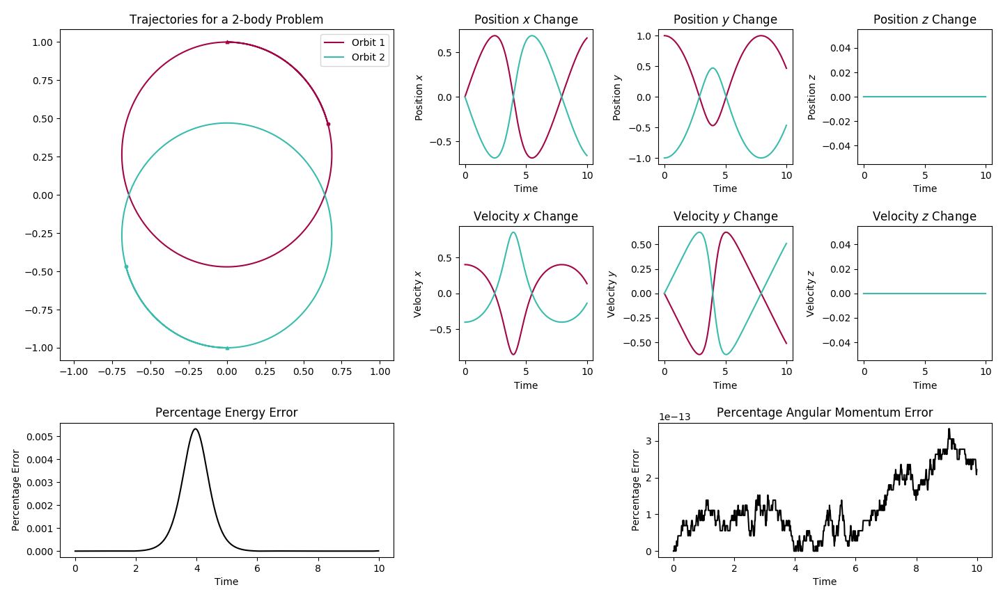
and display the following in terminal:
Bodies: 2
Total Mass: 2
Centre of Mass: [0. 0. 0.]
Linear Momentum:
 [[ 0.4  0.   0. ]
 [-0.4  0.   0. ]]
Total Linear Momentum: [0. 0. 0.]
Angular Momentum:
 [[ 0.   0.  -0.4]
 [-0.  -0.  -0.4]]
Total Angular Momentum: [ 0.   0.  -0.8]
Kinetic Energy: 0.16000000000000003
Gravitational Potential Energy: -0.5
Total Energy: -0.33999999999999997

--------------------

Bodies: 2
Total Mass: 2
Centre of Mass: [0. 0. 0.]
Linear Momentum:
 [[ 0.13593791 -0.51027534  0.        ]
 [-0.13593791  0.51027534  0.        ]]
Total Linear Momentum: [0. 0. 0.]
Angular Momentum:
 [[ 0.   0.  -0.4]
 [-0.   0.  -0.4]]
Total Angular Momentum: [ 0.   0.  -0.8]
Kinetic Energy: 0.27886003434284173
Gravitational Potential Energy: -0.6188600694601704
Total Energy: -0.3400000351173286
How To Get a Stability Image
To produce a Stability Image, you simply need a file from stability_investigation. To calculate the image, use MPStabilityPlotter instead of StabilityPlotter as the former uses Python's multiprocessing to speed up calculations. By default, we perturb a Figure of 8, and use Leapfrog3 with adaptive time step to compute orbits
- Instantiate
MPStabilityPlotter: this requires parameters for the size and number of perturbations, alongside parameters to instantiate the simulations. - Calculate Stability Matrix: simply use the
get_stability_matrix()method of theMPStabilityPlotterinstance. - Display the Stability Matrix: simply use the
plot_stability_matrix()method of theMPStabilityPlotterinstance. You can also specify arguments for the plot (number of ticks, continuous colormap, etc ...), as well as for saving the output (as an image, or as JSON). JSON saving can also be used without plotting via thestability_matrix_to_json()method. If we specifyfig_name = None, it automatically generates a file path using the parameters of the instance.
Alternatively, after instantiating the plotter, running plot_stability_matrix() with stability_matrix = None will automatically calculate the stability matrix and plot it.
For example:
from nbodysim.stability_investigator.mp_stability_plotter import MPStabilityPlotter

mpsp = MPStabilityPlotter(perturb=0.005, n_trials=500, collision_tolerance = 10**-3, escape_tolerance = 10, steps = 10**4, delta = 10**-2, tolerance = 10**-2, adaptive_constant = 0.1, delta_lim = 10**-5)
stability_matrix = mpsp.get_stability_matrix()
mpsp.plot_stability_matrix(stability_matrix, n_ticks = 10, grad = True, show = True, save_fig = True, save_matrix = False, fig_name = None, json_name = "my_json.json")
which produces:
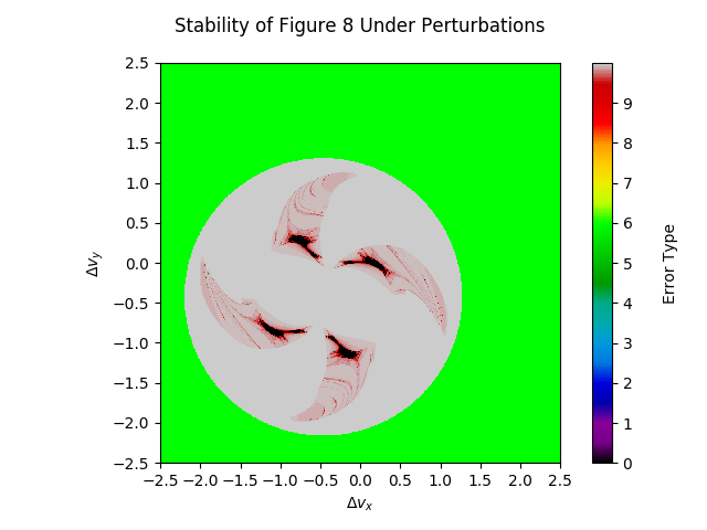
Examples of the stability images, alongside the JSONs they produce can be found in my GitHub repo here.
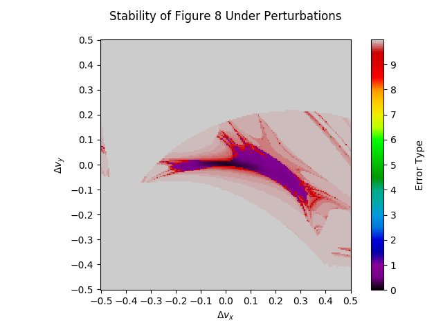
The stability image can be made more interesting by colourising the degree of stability of the stable regions. For this, use StabilityAnalyser The easiest, fastest way of instantiating is by providing a StabilityPlotter alongside the stability_matrix that we want to colourise. Alternatively, we can pass the parameters of a StabilityPlotter alongside the file path to a JSON containing the stability_matrix in order to instantiate. The simplest way to obtain the new image is by running plot_updated_stability_matrix() with sb_scores = None, square_size = 0.01, alongside other arguments like the ones for plot_stability_matrix(). For example:
from nbodysim.stability_investigator.mp_stability_plotter import MPStabilityPlotter
from nbodysim.stability_investigator.stability_analyser importStabilityAnalyser

mpsp = MPStabilityPlotter(perturb=0.005, n_trials=100, collision_tolerance = 10**-3, escape_tolerance = 10, steps = 10**4, delta = 10**-2, tolerance = 10**-2, adaptive_constant = 0.1, delta_lim = 10**-5)
stability_matrix = mpsp.get_stability_matrix()
mpsp_analyser = MPSPAnalyser(mpsp, stability_matrix)
mpsp_analyser.plot_updated_stability_matrix(sb_scores = None, square_size = 0.01, n_ticks = 10, grad = True, show = True, save_fig = False, save_matrix = False, fig_name = "report_imgs/sb_scores_HD")
which under the hood does:
from nbodysim.stability_investigator.mp_stability_plotter import MPStabilityPlotter
from nbodysim.stability_investigator.stability_analyser importStabilityAnalyser

mpsp = MPStabilityPlotter(perturb=0.005, n_trials=100, collision_tolerance = 10**-3, escape_tolerance = 10, steps = 10**4, delta = 10**-2, tolerance = 10**-2, adaptive_constant = 0.1, delta_lim = 10**-5)
stability_matrix = mpsp.get_stability_matrix()
mpsp_analyser = MPSPAnalyser(mpsp, stability_matrix)
mpsp_analyser.update_stability_matrix(sb_scores)
sb_scores = mpsp_analyser.get_stability_scores(0.01)
mpsp_analyser.plot_updated_stability_matrix(n_ticks = 10, grad = True, show = True, save_fig = False, save_matrix = False, fig_name = "report_imgs/sb_scores_HD")
resulting in:
Release history Release notifications | RSS feed


Download files
Download the file for your platform. If you're not sure which to choose, learn more about installing packages.
Source Distribution
Built Distribution
Filter files by name, interpreter, ABI, and platform.
If you're not sure about the file name format, learn more about wheel file names.
Copy a direct link to the current filters
File details
Details for the file nbodysim-1.0.3.tar.gz.
File metadata
- Download URL: nbodysim-1.0.3.tar.gz
- Upload date:
- Size: 28.7 kB
- Tags: Source
- Uploaded using Trusted Publishing? No
- Uploaded via: twine/4.0.0 CPython/3.7.0
File hashes
| Algorithm | Hash digest | |
|---|---|---|
| SHA256 |
88e26398c4bafed9241aeef0980999f15ab29fece41684733a844de071f54d3f
|
|
| MD5 |
8db98445e22e24c5605b84b4a9ffc031
|
|
| BLAKE2b-256 |
3860b6b4802800f3fb33adb9a94f67e9d18ccd5f1a587f27708e945564fcf23d
|
File details
Details for the file nbodysim-1.0.3-py3-none-any.whl.
File metadata
- Download URL: nbodysim-1.0.3-py3-none-any.whl
- Upload date:
- Size: 37.2 kB
- Tags: Python 3
- Uploaded using Trusted Publishing? No
- Uploaded via: twine/4.0.0 CPython/3.7.0
File hashes
| Algorithm | Hash digest | |
|---|---|---|
| SHA256 |
cf9a7ac942aa44b6efd4bafd0ff4ca61f361dd07688a0020b20d347c79d02188
|
|
| MD5 |
32a49927196ea25dccfa1c2be62845a3
|
|
| BLAKE2b-256 |
57df389b84c997c4e1b54e7144ddd6e5424ca185ec6e1da1a06e4a9f9d0c377a
|






