


Neo LS-SVM
Neo LS-SVM is a modern Least-Squares Support Vector Machine implementation in Python that offers several benefits over sklearn's classic sklearn.svm.SVC classifier and sklearn.svm.SVR regressor:
- ⚡ Linear complexity in the number of training examples with Orthogonal Random Features.
- 🚀 Hyperparameter free: zero-cost optimization of the regularisation parameter γ and kernel parameter σ.
- 🏔️ Adds a new tertiary objective that minimizes the complexity of the prediction surface.
- 🎁 Returns the leave-one-out residuals and error for free after fitting.
- 🌀 Learns an affine transformation of the feature matrix to optimally separate the target's bins.
- 🪞 Can solve the LS-SVM both in the primal and dual space.
- 🌡️ Isotonically calibrated
predict_proba. - ✅ Conformally calibrated
predict_quantilesandpredict_interval. - 🔔 Bayesian estimation of the predictive standard deviation with
predict_std. - 🐼 Pandas DataFrame output when the input is a pandas DataFrame.
Using
Installing
First, install this package with:
pip install neo-ls-svm
Classification and regression
Then, you can import neo_ls_svm.NeoLSSVM as an sklearn-compatible binary classifier and regressor. Example usage:
from neo_ls_svm import NeoLSSVM
from pandas import get_dummies
from sklearn.datasets import fetch_openml
from sklearn.model_selection import train_test_split

# Binary classification example:
X, y = fetch_openml("churn", version=3, return_X_y=True, as_frame=True, parser="auto")
X_train, X_test, y_train, y_test = train_test_split(get_dummies(X), y, test_size=0.15, random_state=42)
model = NeoLSSVM().fit(X_train, y_train)
model.score(X_test, y_test)  # 93.1% (compared to sklearn.svm.SVC's 89.6%)

# Regression example:
X, y = fetch_openml("ames_housing", version=1, return_X_y=True, as_frame=True, parser="auto")
X_train, X_test, y_train, y_test = train_test_split(get_dummies(X), y, test_size=0.15, random_state=42)
model = NeoLSSVM().fit(X_train, y_train)
model.score(X_test, y_test)  # 82.4% (compared to sklearn.svm.SVR's -11.8%)
Predicting quantiles
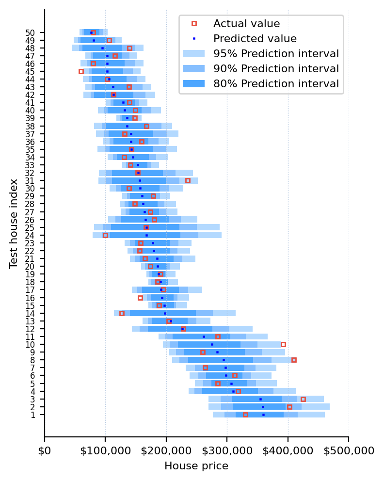
Neo LS-SVM implements conformal prediction with a Bayesian nonconformity estimate to compute quantiles and prediction intervals for both classification and regression. Example usage:
# Predict the house prices and their quantiles.
ŷ_test = model.predict(X_test)
ŷ_test_quantiles = model.predict_quantiles(X_test, quantiles=(0.025, 0.05, 0.1, 0.9, 0.95, 0.975))
When the input data is a pandas DataFrame, the output is also a pandas DataFrame. For example, printing the head of ŷ_test_quantiles yields:
| house_id | 0.025 | 0.05 | 0.1 | 0.9 | 0.95 | 0.975 |
|---|---|---|---|---|---|---|
| 1357 | 114283.0 | 124767.6 | 133314.0 | 203162.0 | 220407.5 | 245655.3 |
| 2367 | 85518.3 | 91787.2 | 93709.8 | 107464.3 | 108472.6 | 114482.3 |
| 2822 | 147165.9 | 157462.8 | 167193.1 | 243646.5 | 263324.4 | 291963.3 |
| 2126 | 81788.7 | 88738.1 | 91367.4 | 111944.9 | 114800.7 | 122874.5 |
| 1544 | 94507.1 | 108288.2 | 120184.3 | 222630.5 | 248668.2 | 283703.4 |
Let's visualize the predicted quantiles on the test set:
Expand to see the code that generated the graph above
import matplotlib.pyplot as plt
import matplotlib.ticker as ticker

%config InlineBackend.figure_format = "retina"
plt.rcParams["font.size"] = 8
idx = (-ŷ_test.sample(50, random_state=42)).sort_values().index
y_ticks = list(range(1, len(idx) + 1))
plt.figure(figsize=(4, 5))
for j in range(3):
    end = ŷ_test_quantiles.shape[1] - 1 - j
    coverage = round(100 * (ŷ_test_quantiles.columns[end] - ŷ_test_quantiles.columns[j]))
    plt.barh(
        y_ticks,
        ŷ_test_quantiles.loc[idx].iloc[:, end] - ŷ_test_quantiles.loc[idx].iloc[:, j],
        left=ŷ_test_quantiles.loc[idx].iloc[:, j],
        label=f"{coverage}% Prediction interval",
        color=["#b3d9ff", "#86bfff", "#4da6ff"][j],
    )
plt.plot(y_test.loc[idx], y_ticks, "s", markersize=3, markerfacecolor="none", markeredgecolor="#e74c3c", label="Actual value")
plt.plot(ŷ_test.loc[idx], y_ticks, "s", color="blue", markersize=0.6, label="Predicted value")
plt.xlabel("House price")
plt.ylabel("Test house index")
plt.xlim(0, 500e3)
plt.yticks(y_ticks, y_ticks)
plt.tick_params(axis="y", labelsize=6)
plt.grid(axis="x", color="lightsteelblue", linestyle=":", linewidth=0.5)
plt.gca().xaxis.set_major_formatter(ticker.StrMethodFormatter("${x:,.0f}"))
plt.gca().spines["top"].set_visible(False)
plt.gca().spines["right"].set_visible(False)
plt.legend()
plt.tight_layout()
plt.show()
Predicting intervals
In addition to quantile prediction, you can use predict_interval to predict conformally calibrated prediction intervals. Compared to quantiles, these focus on reliable coverage over quantile accuracy. Example usage:
# Compute prediction intervals for the houses in the test set.
ŷ_test_interval = model.predict_interval(X_test, coverage=0.95)

# Measure the coverage of the prediction intervals on the test set
coverage = ((ŷ_test_interval.iloc[:, 0] <= y_test) & (y_test <= ŷ_test_interval.iloc[:, 1])).mean()
print(coverage)  # 94.3%
When the input data is a pandas DataFrame, the output is also a pandas DataFrame. For example, printing the head of ŷ_test_interval yields:
| house_id | 0.025 | 0.975 |
|---|---|---|
| 1357 | 114283.0 | 245849.2 |
| 2367 | 85518.3 | 114411.4 |
| 2822 | 147165.9 | 292179.2 |
| 2126 | 81788.7 | 122838.1 |
| 1544 | 94507.1 | 284062.6 |
Benchmarks
We select all binary classification and regression datasets below 1M entries from the AutoML Benchmark. Each dataset is split into 85% for training and 15% for testing. We apply skrub.TableVectorizer as a preprocessing step for neo_ls_svm.NeoLSSVM and sklearn.svm.SVC,SVR to vectorize the pandas DataFrame training data into a NumPy array. Models are fitted only once on each dataset, with their default settings and no hyperparameter tuning.
Binary classification
ROC-AUC on 15% test set:
| dataset | LGBMClassifier | NeoLSSVM | SVC |
|---|---|---|---|
| ada | 🥈 90.9% (0.1s) | 🥇 90.9% (1.9s) | 83.1% (4.5s) |
| adult | 🥇 93.0% (0.5s) | 🥈 89.0% (15.7s) | / |
| amazon_employee_access | 🥇 85.6% (0.5s) | 🥈 64.5% (9.0s) | / |
| arcene | 🥈 78.0% (0.6s) | 70.0% (6.3s) | 🥇 82.0% (4.0s) |
| australian | 🥇 88.3% (0.2s) | 79.9% (1.7s) | 🥈 81.9% (0.1s) |
| bank-marketing | 🥇 93.5% (0.5s) | 🥈 91.0% (11.8s) | / |
| blood-transfusion-service-center | 62.0% (0.3s) | 🥇 71.0% (2.2s) | 🥈 69.7% (0.1s) |
| churn | 🥇 91.7% (0.6s) | 🥈 81.0% (2.1s) | 70.6% (2.9s) |
| click_prediction_small | 🥇 67.7% (0.5s) | 🥈 66.6% (10.9s) | / |
| jasmine | 🥇 86.1% (0.3s) | 79.5% (1.9s) | 🥈 85.3% (7.4s) |
| kc1 | 🥇 78.9% (0.3s) | 🥈 76.6% (1.4s) | 45.7% (0.6s) |
| kr-vs-kp | 🥇 100.0% (0.6s) | 99.2% (1.6s) | 🥈 99.4% (2.3s) |
| madeline | 🥇 93.1% (0.5s) | 65.6% (1.9s) | 🥈 82.5% (19.8s) |
| ozone-level-8hr | 🥈 91.2% (0.4s) | 🥇 91.6% (1.7s) | 72.9% (0.6s) |
| pc4 | 🥇 95.3% (0.3s) | 🥈 90.9% (1.5s) | 25.7% (0.3s) |
| phishingwebsites | 🥇 99.5% (0.5s) | 🥈 98.9% (3.6s) | 98.7% (10.0s) |
| phoneme | 🥇 95.6% (0.3s) | 🥈 93.5% (2.1s) | 91.2% (2.0s) |
| qsar-biodeg | 🥇 92.7% (0.4s) | 🥈 91.1% (5.2s) | 86.8% (0.3s) |
| satellite | 🥈 98.7% (0.2s) | 🥇 99.5% (1.9s) | 98.5% (0.4s) |
| sylvine | 🥇 98.5% (0.2s) | 🥈 97.1% (2.0s) | 96.5% (3.8s) |
| wilt | 🥈 99.5% (0.2s) | 🥇 99.8% (1.8s) | 98.9% (0.5s) |
Regression
R² on 15% test set:
| dataset | LGBMRegressor | NeoLSSVM | SVR |
|---|---|---|---|
| abalone | 🥈 56.2% (0.1s) | 🥇 59.5% (2.5s) | 51.3% (0.7s) |
| boston | 🥇 91.7% (0.2s) | 🥈 89.6% (1.1s) | 35.1% (0.0s) |
| brazilian_houses | 🥈 55.9% (0.3s) | 🥇 88.4% (3.7s) | 5.4% (7.0s) |
| colleges | 🥇 58.5% (0.4s) | 🥈 42.2% (6.6s) | 40.2% (15.1s) |
| diamonds | 🥇 98.2% (0.3s) | 🥈 95.2% (13.7s) | / |
| elevators | 🥇 87.7% (0.5s) | 🥈 82.6% (6.5s) | / |
| house_16h | 🥇 67.7% (0.4s) | 🥈 52.8% (6.0s) | / |
| house_prices_nominal | 🥇 89.0% (0.3s) | 🥈 78.3% (2.1s) | -2.9% (1.2s) |
| house_sales | 🥇 89.2% (0.4s) | 🥈 77.8% (5.9s) | / |
| mip-2016-regression | 🥇 59.2% (0.4s) | 🥈 34.9% (5.8s) | -27.3% (0.4s) |
| moneyball | 🥇 93.2% (0.3s) | 🥈 91.3% (1.1s) | 0.8% (0.2s) |
| pol | 🥇 98.7% (0.3s) | 🥈 74.9% (4.6s) | / |
| quake | -10.7% (0.2s) | 🥇 -1.0% (1.6s) | 🥈 -10.7% (0.1s) |
| sat11-hand-runtime-regression | 🥇 78.3% (0.4s) | 🥈 61.7% (2.1s) | -56.3% (5.1s) |
| sensory | 🥇 29.2% (0.1s) | 3.0% (1.6s) | 🥈 16.4% (0.0s) |
| socmob | 🥇 79.6% (0.2s) | 🥈 72.5% (6.6s) | 30.8% (0.1s) |
| space_ga | 🥇 70.3% (0.3s) | 🥈 43.6% (1.5s) | 35.9% (0.2s) |
| tecator | 🥈 98.3% (0.1s) | 🥇 99.4% (0.9s) | 78.5% (0.0s) |
| us_crime | 🥈 62.8% (0.6s) | 🥇 63.0% (2.3s) | 6.7% (0.8s) |
| wine_quality | 🥇 45.6% (0.2s) | 🥈 36.5% (2.8s) | 16.4% (1.6s) |
Contributing
Prerequisites
1. Set up Git to use SSH
- Generate an SSH key and add the SSH key to your GitHub account.
- Configure SSH to automatically load your SSH keys:
cat << EOF >> ~/.ssh/config
Host *
  AddKeysToAgent yes
  IgnoreUnknown UseKeychain
  UseKeychain yes
EOF
2. Install Docker
- Install Docker Desktop.
- Enable Use Docker Compose V2 in Docker Desktop's preferences window.
- Linux only:
- Export your user's user id and group id so that files created in the Dev Container are owned by your user:
cat << EOF >> ~/.bashrc
export UID=$(id --user)
export GID=$(id --group)
EOF
- Export your user's user id and group id so that files created in the Dev Container are owned by your user:
3. Install VS Code or PyCharm
- Install VS Code and VS Code's Dev Containers extension. Alternatively, install PyCharm.
- Optional: install a Nerd Font such as FiraCode Nerd Font and configure VS Code or configure PyCharm to use it.
Development environments
The following development environments are supported:
- ⭐️ GitHub Codespaces: click on Code and select Create codespace to start a Dev Container with GitHub Codespaces.
- ⭐️ Dev Container (with container volume): click on Open in Dev Containers to clone this repository in a container volume and create a Dev Container with VS Code.
- Dev Container: clone this repository, open it with VS Code, and run Ctrl/⌘ + ⇧ + P → Dev Containers: Reopen in Container.
- PyCharm: clone this repository, open it with PyCharm, and configure Docker Compose as a remote interpreter with the
devservice. - Terminal: clone this repository, open it with your terminal, and run
docker compose up --detach devto start a Dev Container in the background, and then rundocker compose exec dev zshto open a shell prompt in the Dev Container.
Developing
- This project follows the Conventional Commits standard to automate Semantic Versioning and Keep A Changelog with Commitizen.
- Run
poefrom within the development environment to print a list of Poe the Poet tasks available to run on this project. - Run
poetry add {package}from within the development environment to install a run time dependency and add it topyproject.tomlandpoetry.lock. Add--group testor--group devto install a CI or development dependency, respectively. - Run
poetry updatefrom within the development environment to upgrade all dependencies to the latest versions allowed bypyproject.toml. - Run
cz bumpto bump the package's version, update theCHANGELOG.md, and create a git tag.
1 maintainer

Release files for neo-ls-svm 0.3.0
For a detailed explanation of source distributions (sdists) and built distributions (wheels), please see the package formats documentation.
Source distribution (sdist)
| File | Size | Uploaded | |
|---|---|---|---|
| neo_ls_svm-0.3.0.tar.gz | 37.2 kB | Details |
Built distribution (wheel)
| File | Interpreter | ABI | Platform | Reset |
|---|---|---|---|---|
| neo_ls_svm-0.3.0-py3-none-any.whl | Python 3 | none | any | Details |
Total release size: 73.2 kB
Release files / neo_ls_svm-0.3.0.tar.gz
| Download URL | neo_ls_svm-0.3.0.tar.gz |
|---|---|
| Size | 37.2 kB |
| Tags | Source |
|
SHA-256 checksum How to use checksums |
e92baa007479b8746630c4d2acea1d6740fde34d08eb79dce081e4541dfc39b4
|
|
BLAKE2b-256 checksum How to use checksums |
82fc4c4b97e7a5a3faec5e321d251b50c62582b07f4d7c1d1bd2d14ee2adc4c1
|
| Upload date | |
|
Uploaded using Trusted Publishing? What is trusted publishing? |
No |
| Uploaded via |
poetry/1.8.2 CPython/3.10.14 Linux/6.5.0-1016-azure
|
Release files / neo_ls_svm-0.3.0-py3-none-any.whl
| Download URL | neo_ls_svm-0.3.0-py3-none-any.whl |
|---|---|
| Size | 36.1 kB |
| Tags | Python 3 |
|
SHA-256 checksum How to use checksums |
be8680bf598726535c96cdd1aa79cc594ce3ac85f21d4b3d40f9e868af7e5998
|
|
BLAKE2b-256 checksum How to use checksums |
ea1f9dc52cb21b58b914c5c90e616c786a47e1058ec1a1cf3c0cd01ea6ed35ba
|
| Upload date | |
|
Uploaded using Trusted Publishing? What is trusted publishing? |
No |
| Uploaded via |
poetry/1.8.2 CPython/3.10.14 Linux/6.5.0-1016-azure
|














