A high-performance library for building Neutral Landscape Models
Verified details
These details have been verified by PyPIProject links
GitHub Statistics
Maintainers

Project description
nlmrs
A Rust crate for building Neutral Landscape Models.
nlmrs is available as a Rust crate or as a CLI tool. Language bindings are also provided for Python, R, Julia, WASM, and C.
Installation
cargo add nlmrs
Example
use nlmrs;

fn main() {
    let arr = nlmrs::midpoint_displacement(10, 10, 1.);
    println!("{:?}", arr);

    nlmrs::export::write_to_csv(arr, "./data.csv");
}
Algorithms
Gradient
Deterministic spatial fields derived from direction, distance, or position.
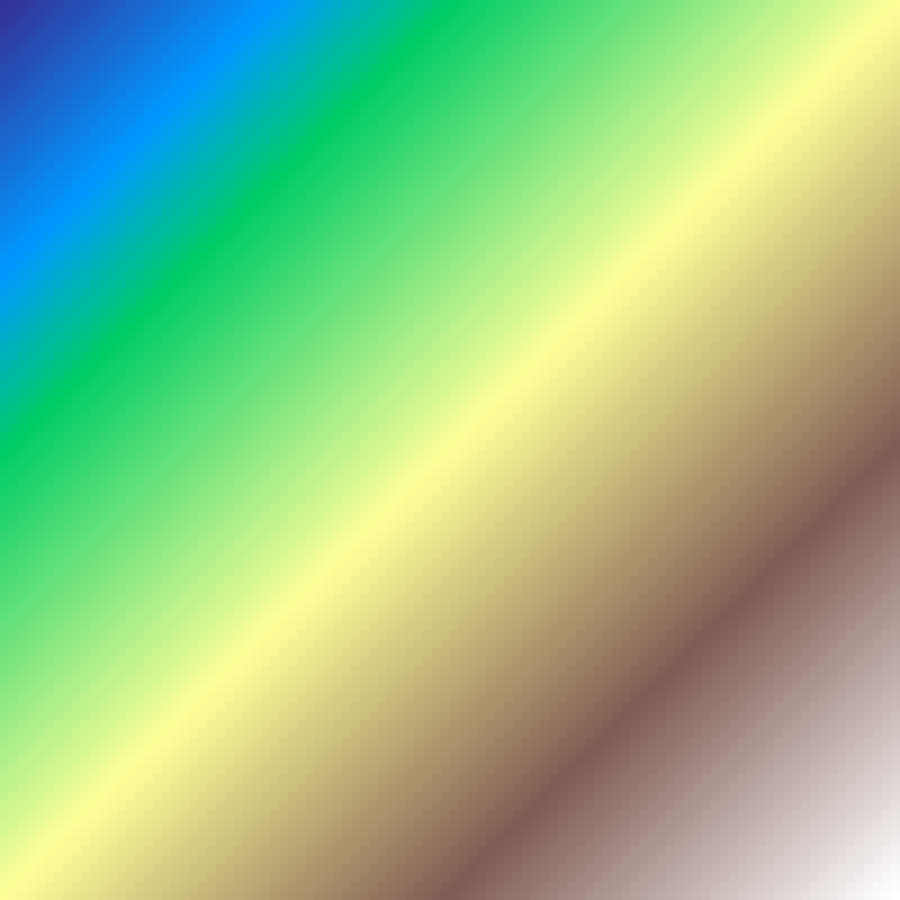
Planar Gradient
planar_gradient(rows: 100, cols: 100, direction: 45.0, seed: 42)
Linear ramp at a given direction angle, increasing uniformly from 0 to 1 across the grid.
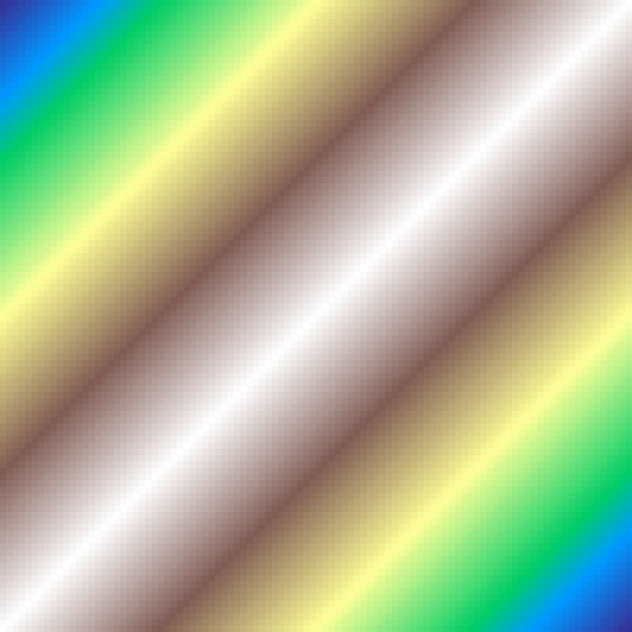
Edge Gradient
edge_gradient(rows: 100, cols: 100, direction: 45.0, seed: 42)
Symmetric version of the planar gradient: values peak at 1.0 along the central axis and fall to 0.0 at both edges.
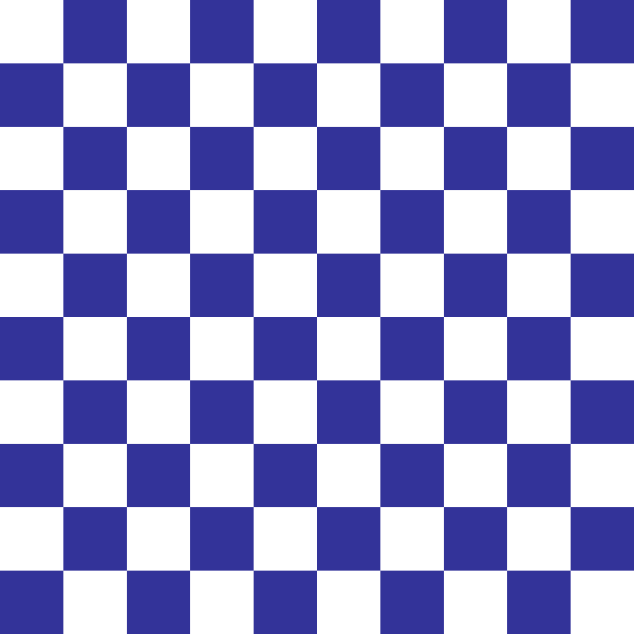
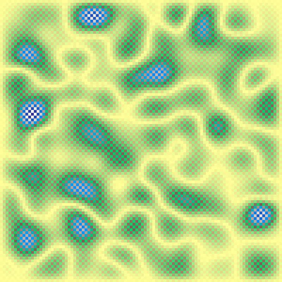
Checkerboard
checkerboard(rows: 100, cols: 100, scale: 10, seed: 42)
Deterministic alternating binary pattern of axis-aligned squares with side length scale cells. Canonical control landscape for spatial autocorrelation analysis.
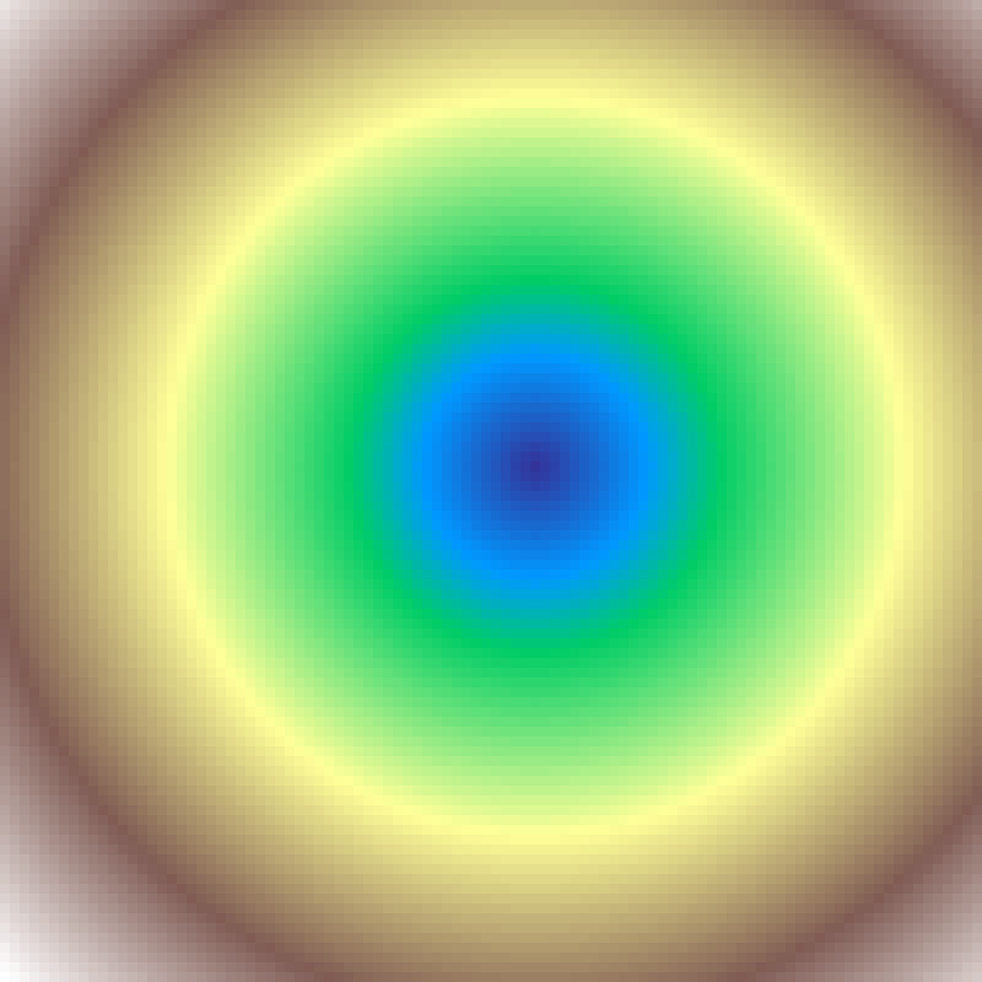
Distance Gradient
distance_gradient(rows: 100, cols: 100, seed: 42)
Euclidean distance transform from random seed cells, producing a smooth radial falloff from 0 at the seeds outward to 1 at the most distant point.
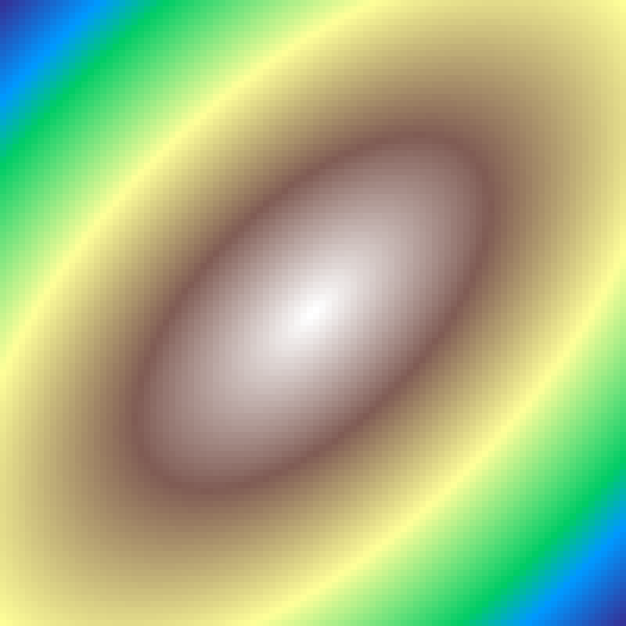
Landscape Gradient
landscape_gradient(rows: 100, cols: 100, direction: 45.0, aspect: 2.0, seed: 42)
Elliptical gradient centred at the grid midpoint. direction orients the major axis; aspect controls elongation (1.0 = circular). More flexible than distance_gradient.
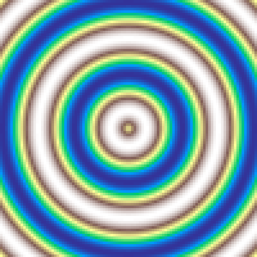
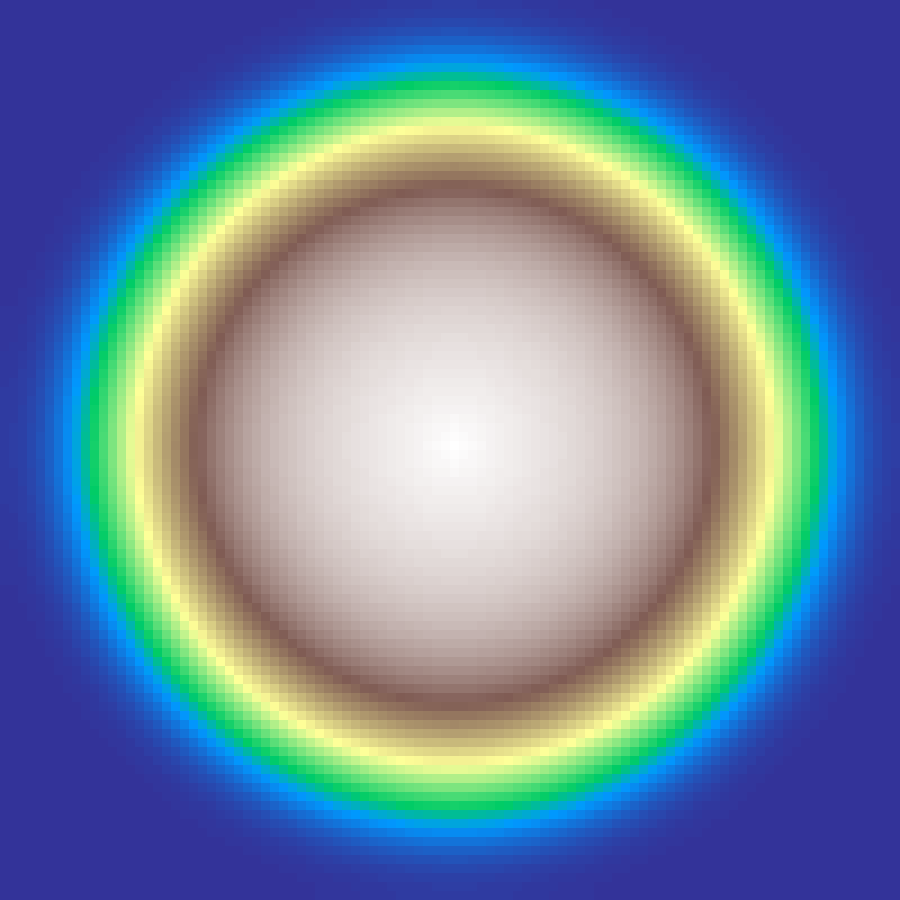
Concentric Rings
concentric_rings(rows: 100, cols: 100, frequency: 5.0, seed: 42)
Sinusoidal rings centred at the grid midpoint. frequency controls how many oscillations span the grid radius; higher values produce tighter, more closely-spaced rings.
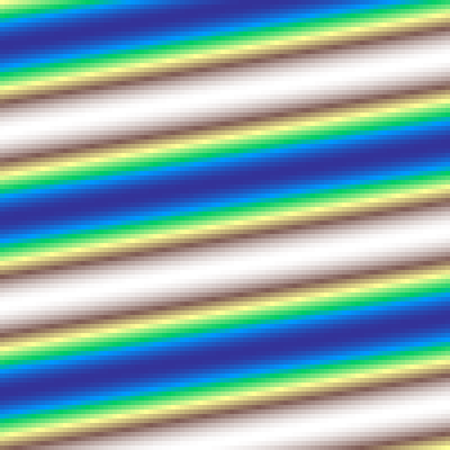
Wave Gradient
wave_gradient(rows: 100, cols: 100, period: 3.0, seed: 42)
Sinusoidal wave oriented at a given direction angle, cycling repeatedly from 0 to 1 and back at the specified period.
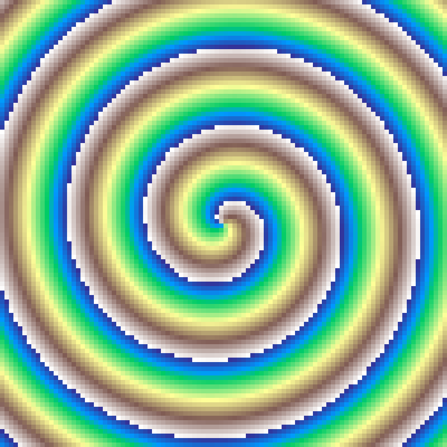
Spiral Gradient
spiral_gradient(rows: 100, cols: 100, turns: 4.0, seed: 42)
Archimedean spiral radiating outward from the grid centre. Values increase along the spiral arms; turns controls how many full rotations span the grid radius.
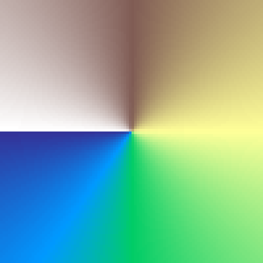
Radial Sweep
radial_sweep(rows: 100, cols: 100, seed: 42)
Deterministic gradient encoding the clockwise angle from the grid centre. Values range from 0 at the top (north) through 0.5 at the bottom, back to 1 at the top, mapping the full 360-degree sweep to [0, 1].
Noise
Continuous stochastic fields, from single-layer lattice noise to multi-octave fractal composites.
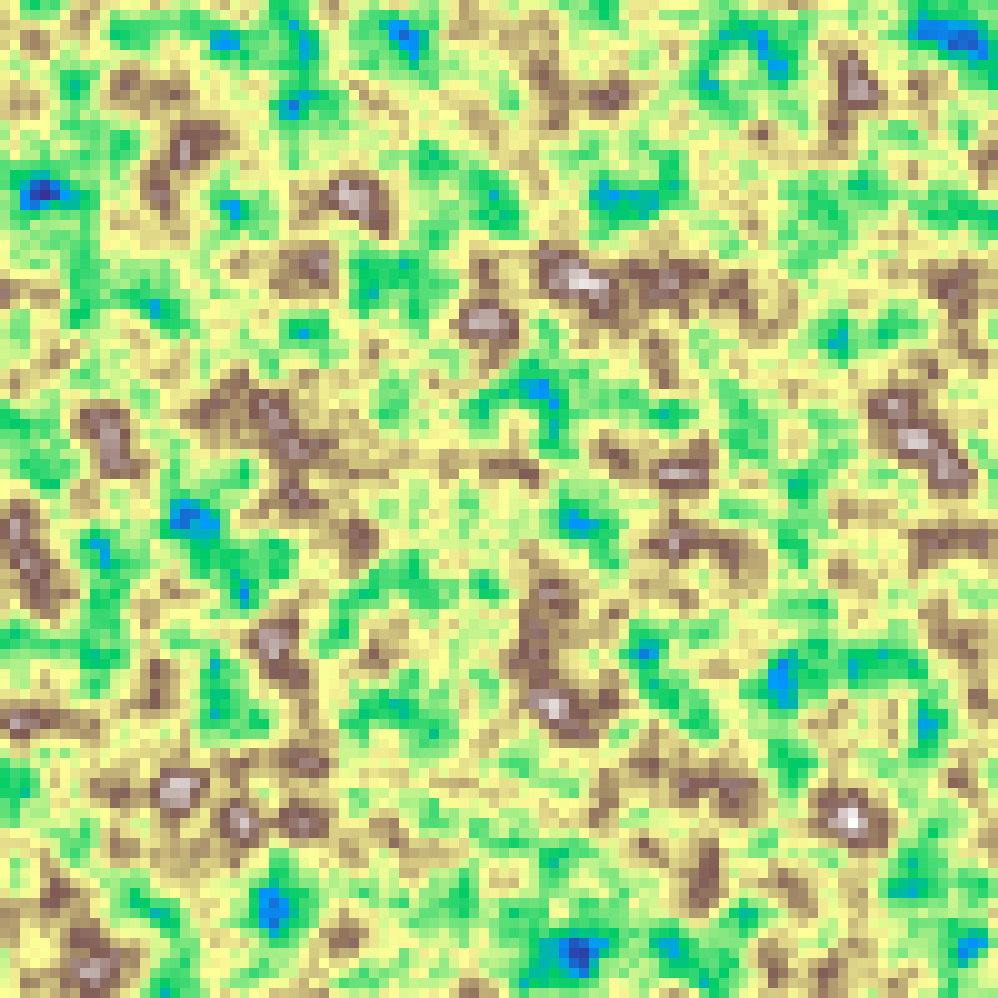
Perlin Noise
perlin_noise(rows: 100, cols: 100, scale: 4.0, seed: 42)
Smooth gradient noise built from dot products of random gradient vectors at lattice points, producing continuous, natural-looking variation.
Source: Perlin (1985)
Simplex Noise
simplex_noise(rows: 100, cols: 100, scale: 4.0, seed: 42)
An open-source alternative to Perlin noise with fewer directional artefacts.
Value Noise
value_noise(rows: 100, cols: 100, scale: 4.0, seed: 42)
Interpolated lattice noise that is smoother and more rounded than Perlin noise.
Worley Noise
worley_noise(rows: 100, cols: 100, scale: 4.0, seed: 42)
Cell noise built from distances to random feature points, producing cellular, cracked-earth, or mosaic-like patterns.
Source: Worley (1996)
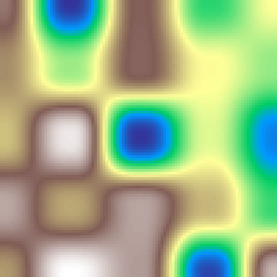
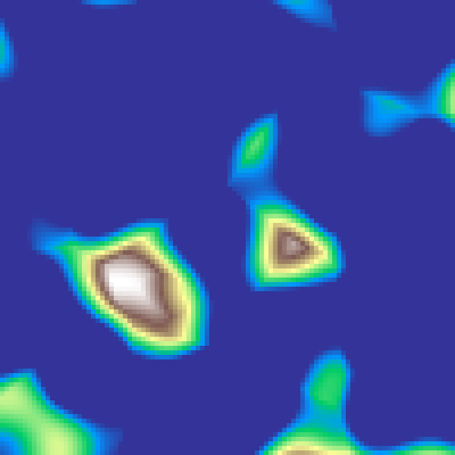
Voronoi Distance
voronoi_distance(rows: 100, cols: 100, n: 50, seed: 42)
Scatters n random feature points across the grid and fills each cell with the Euclidean distance to the nearest point, producing smooth conical gradients centred on each point.
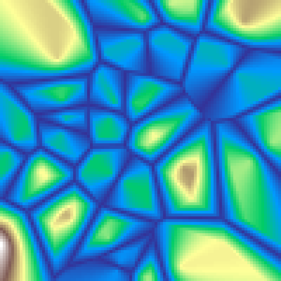
Voronoi Crease
voronoi_crease(rows: 100, cols: 100, n: 30, seed: 42)
F2-F1 Worley noise: the difference between distances to the two nearest seed points. Values peak at Voronoi cell boundaries and fall off toward cell centres, highlighting the skeleton of the Voronoi diagram.
Perlin-Worley Noise
perlin_worley(rows: 100, cols: 100, scale: 4.0, seed: 42)
Hybrid of Perlin and Worley noise computed on the same cell grid. Perlin values are blended with inverted Worley distances, producing fluffy, cloud-like structures with soft cellular interiors.
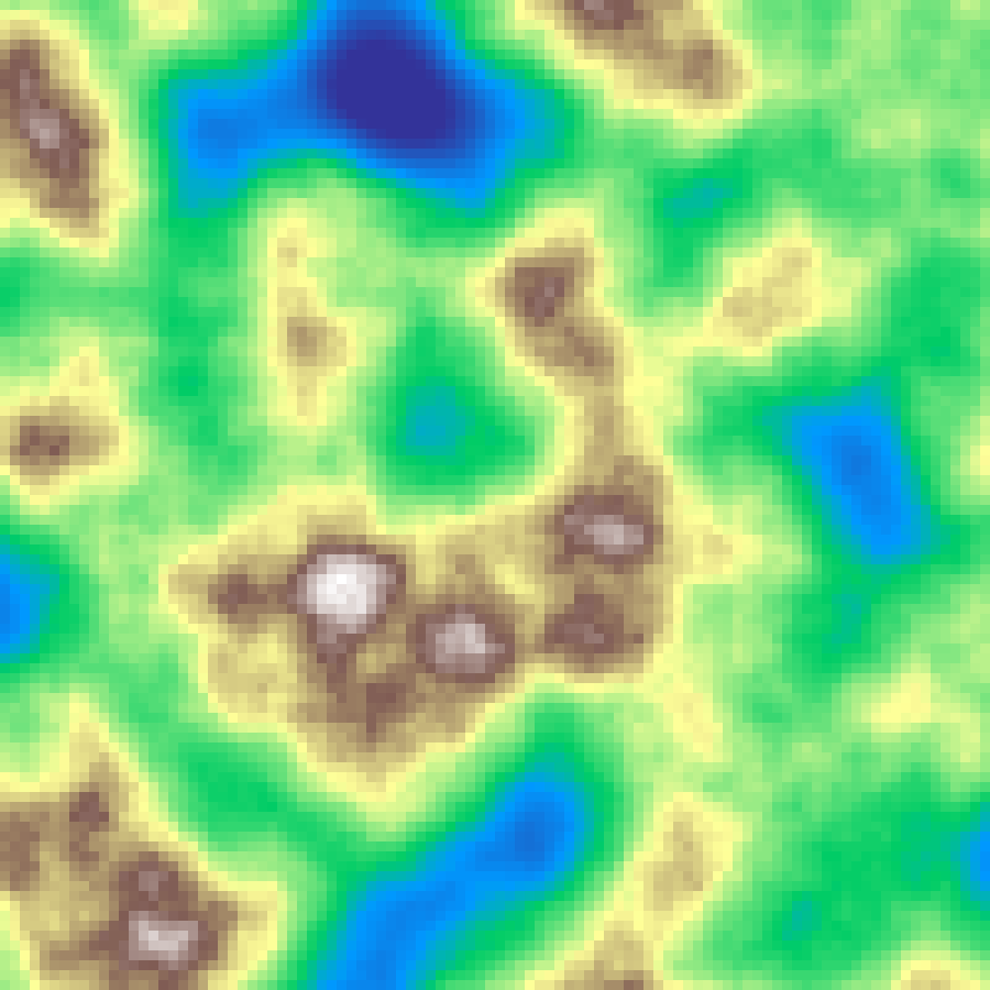
fBm Noise
fbm_noise(rows: 100, cols: 100, scale: 4.0, octaves: 6, seed: 42)
Fractal Brownian motion layers multiple octaves of Perlin noise for more natural-looking terrain detail.
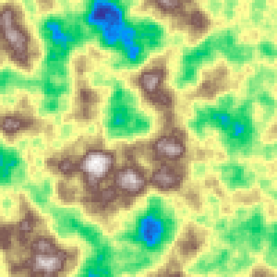
Source: Mandelbrot & Van Ness (1968); Voss (1985)
Ridged Noise
ridged_noise(rows: 100, cols: 100, scale: 4.0, octaves: 6, seed: 42)
Multi-octave noise where each octave is inverted and folded, producing sharp mountain ridges and valleys.
Source: Musgrave, Kolb & Mace (1989)
Billow Noise
billow_noise(rows: 100, cols: 100, scale: 4.0, octaves: 6, seed: 42)
Multi-octave noise with absolute-value folding applied before accumulation, producing rounded billowing clouds or rolling dune shapes.
Source: Ebert et al., Texturing and Modeling: A Procedural Approach (2002)
Hybrid Noise
hybrid_noise(rows: 100, cols: 100, scale: 4.0, octaves: 6, seed: 42)
Hybrid multifractal noise combines fBm-style layering with a multiplicative weighting that amplifies high-frequency detail near peaks.
Source: Musgrave, Kolb & Mace (1989)
Turbulence
turbulence(rows: 100, cols: 100, scale: 4.0, octaves: 6, seed: 42)
fBm with absolute-value folding per octave, producing sharp ridges and a storm-cloud appearance.

Source: Perlin (1985)
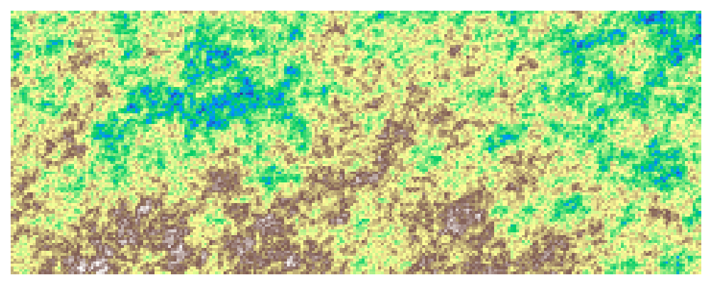
Multifractal Terrain
multifractal_terrain(rows: 100, cols: 100, scale: 4.0, octaves: 6, seed: 42)
Musgrave's heterogeneous multifractal: each successive octave is weighted by the accumulated signal, so low-lying areas remain smooth while ridges and peaks accumulate rugged fine detail. Produces terrain with realistic geological stratification.
Source: Musgrave et al. (1989)
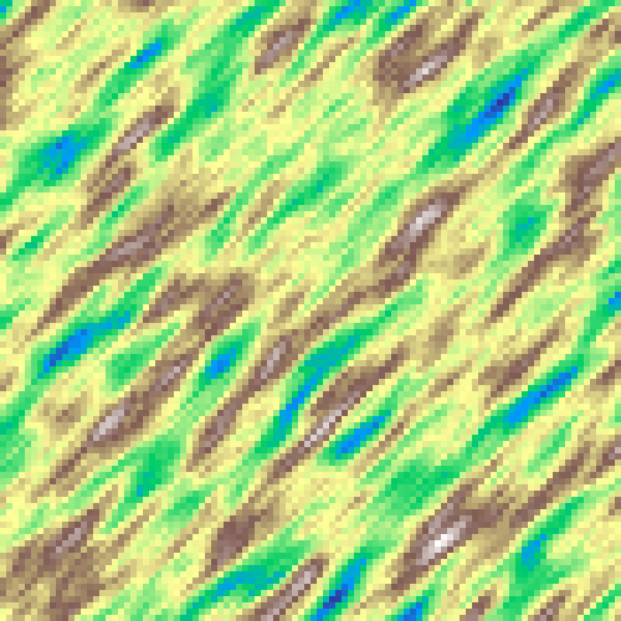
Anisotropic Noise
anisotropic_noise(rows: 100, cols: 100, scale: 4.0, octaves: 6, direction: 45.0, stretch: 4.0, seed: 42)
Fractal Brownian motion computed in a rotated and stretched coordinate frame, producing directionally biased textures. direction sets the elongation axis; stretch controls the anisotropy ratio.
Domain Warp
domain_warp(rows: 100, cols: 100, scale: 4.0, warp_strength: 1.0, seed: 42)
Perlin noise sampled at coordinates displaced by a second Perlin field, producing organic swirling patterns.
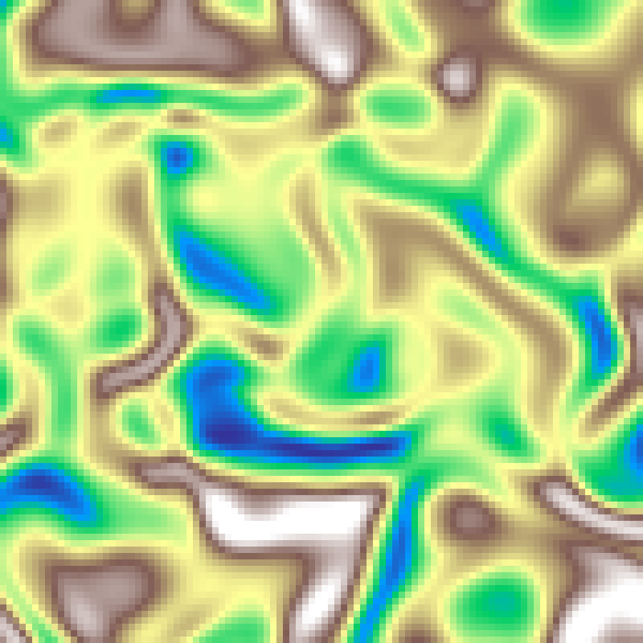
Source: Quilez (2002)
Tiled Noise
tiled_noise(rows: 100, cols: 100, scale: 4.0, seed: 42)
Seamlessly tileable Perlin noise generated by embedding the grid on a 4D torus, ensuring that the left/right and top/bottom edges match perfectly.
Curl Noise
curl_noise(rows: 100, cols: 100, scale: 4.0, seed: 42)
Computes the curl (gradient rotated 90 degrees) of a Perlin potential field using finite differences, producing a divergence-free velocity field. Sample coordinates of a second Perlin generator are warped by this field, yielding swirling, flow-aligned patterns without directional clumping.
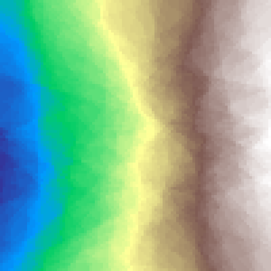
Spectral Synthesis
spectral_synthesis(rows: 100, cols: 100, beta: 2.0, seed: 42)
Generates correlated noise in the frequency domain by scaling each component's amplitude by f^(-beta/2), giving a power spectrum proportional to 1/f^beta. Higher beta produces smoother, more spatially correlated landscapes.
Source: Peitgen & Saupe (1988)
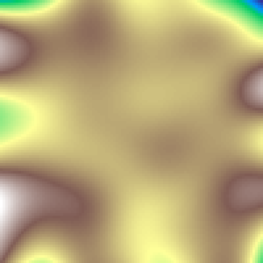
Fractal Brownian Surface
fractal_brownian_surface(rows: 100, cols: 100, h: 0.5, seed: 42)
Spectral synthesis parameterised by the Hurst exponent h ∈ (0, 1), which has direct ecological meaning. h near 0 is rough; h near 1 is smooth. Related to spectral_synthesis by β = 2h + 2.
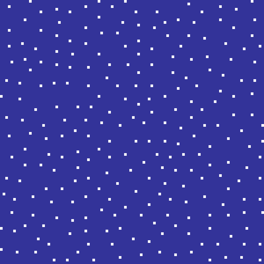
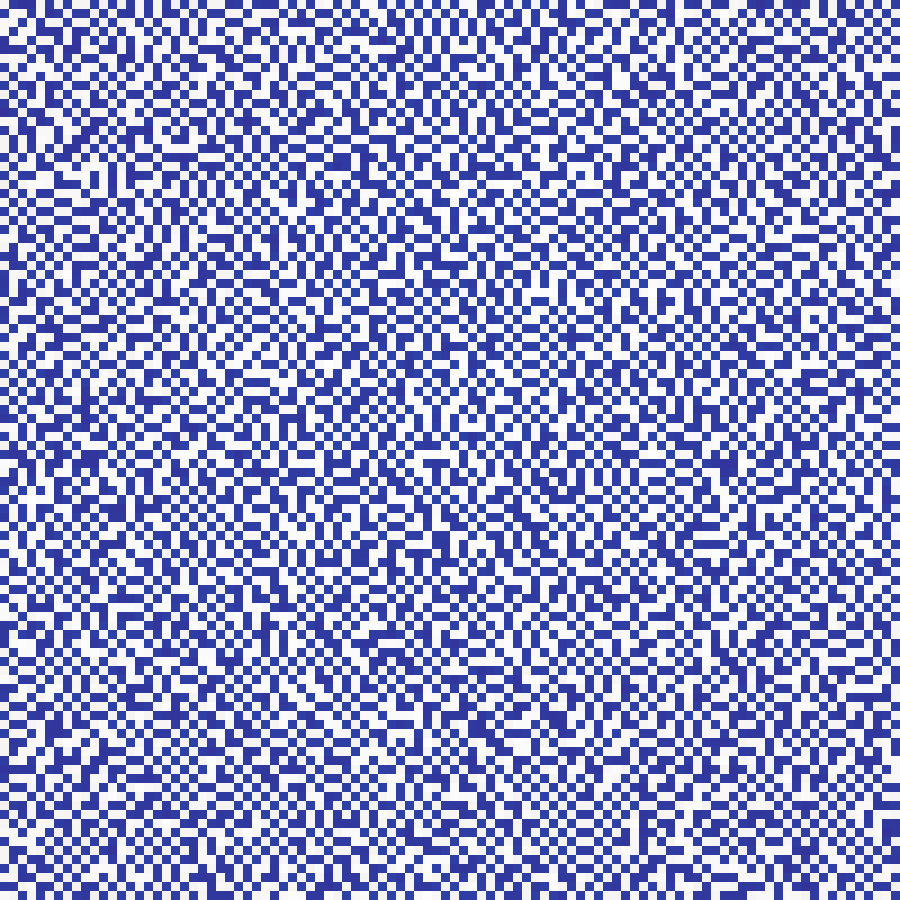
Blue Noise
blue_noise(rows: 100, cols: 100, seed: 42)
Spectral noise with energy concentrated at high spatial frequencies. Generated via FFT by assigning amplitudes proportional to wavenumber magnitude and random phases, then transforming back to the spatial domain. Produces visually uniform, near-Poisson point distributions.
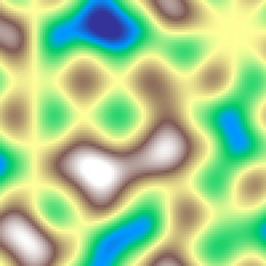
Sine Composite
sine_composite(rows: 100, cols: 100, waves: 8, seed: 42)
Superposes waves sinusoidal plane waves, each with a random orientation, frequency, and phase. The interference of multiple waves produces standing-wave patterns whose complexity grows with the number of waves.
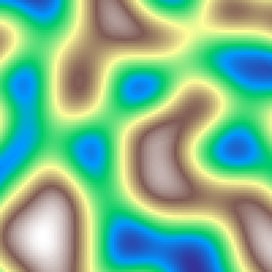
Gabor Noise
gabor_noise(rows: 100, cols: 100, scale: 4.0, n: 500, seed: 42)
Sums n random Gabor kernels (Gaussian-windowed sinusoidal patches) over the grid. Each kernel has a random centre, orientation, and phase; the result is a spatially correlated texture whose dominant frequency is controlled by scale.
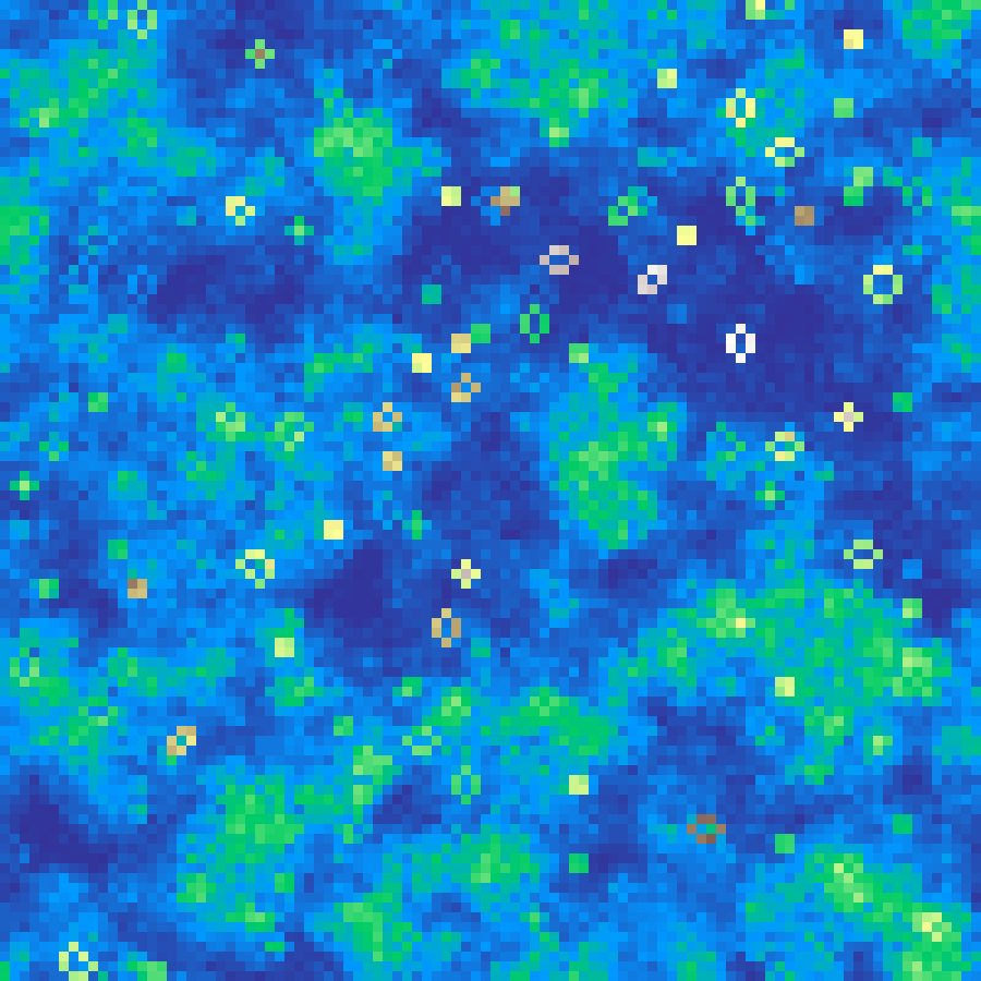
Spot Noise
spot_noise(rows: 100, cols: 100, n: 200, seed: 42)
Places n random elliptical Gaussian spots on the grid, each with an independent orientation, major radius, and aspect ratio. The superimposed spots produce an anisotropic, texture-like field.
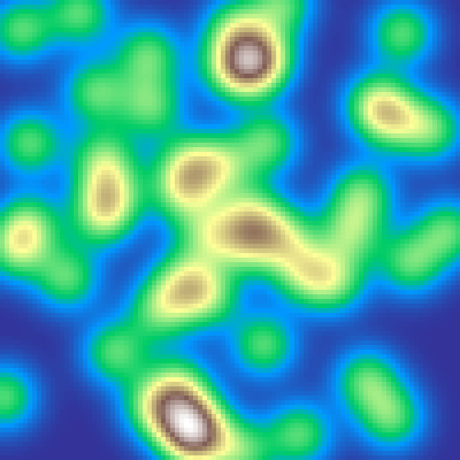
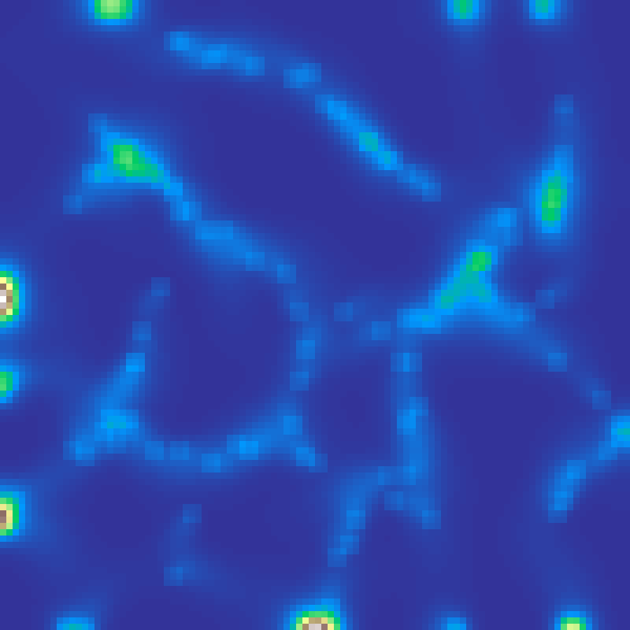
Lognormal Field
lognormal_field(rows: 100, cols: 100, sigma: 10.0, seed: 42)
Gaussian random field transformed by an exponential, giving a right-skewed distribution with rare intense hotspots embedded in a low-value background, typical of ecological quantities such as resource concentrations and population densities.
Patch
Discrete spatial patterns built from random processes, clustering, or hierarchical partitioning.
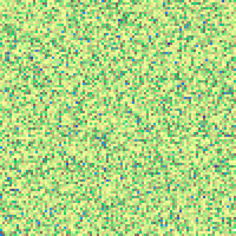
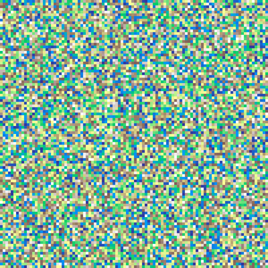
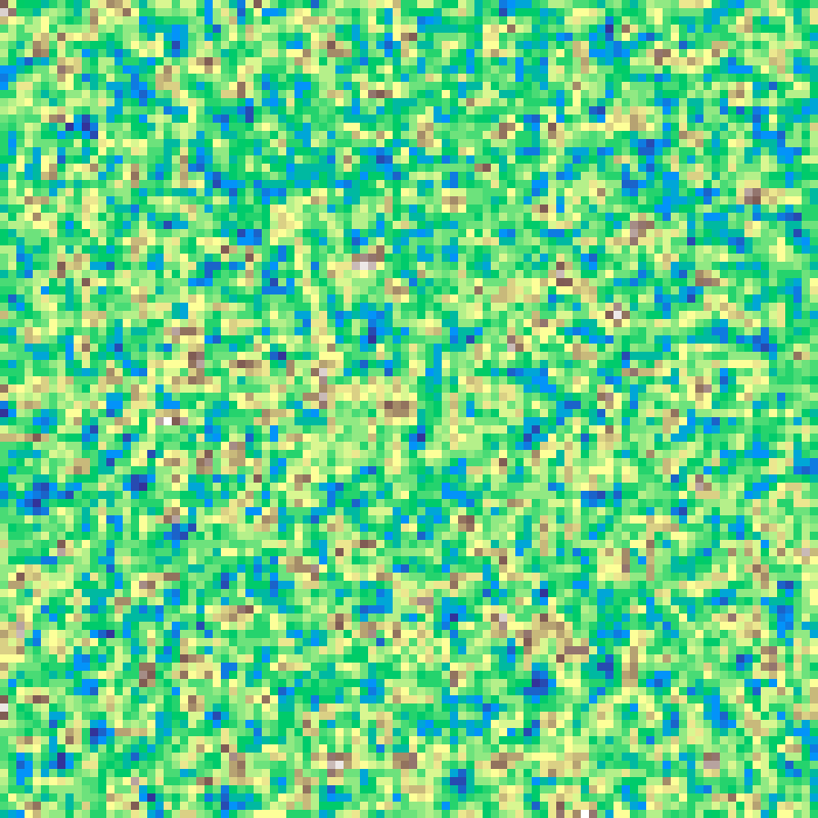
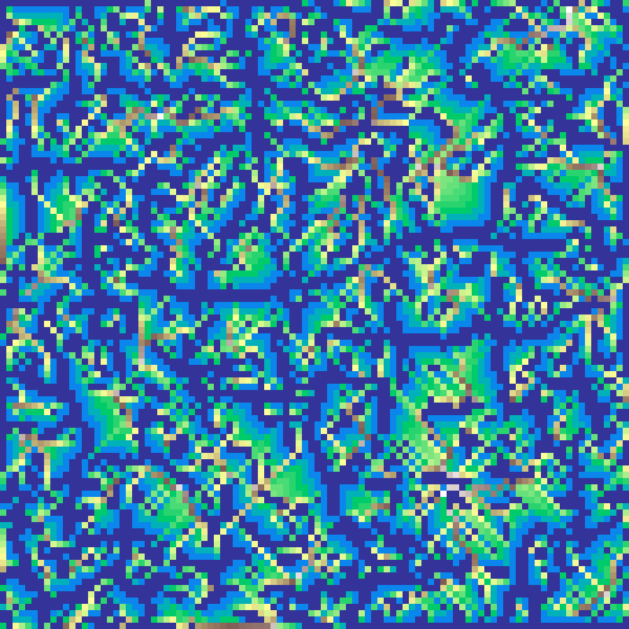
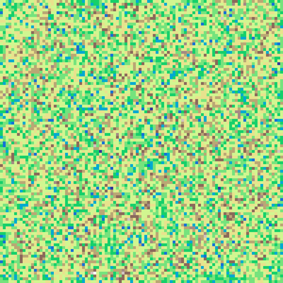
Random
random(rows: 100, cols: 100, seed: 42)
Independent uniform random values at each cell, with no spatial structure.
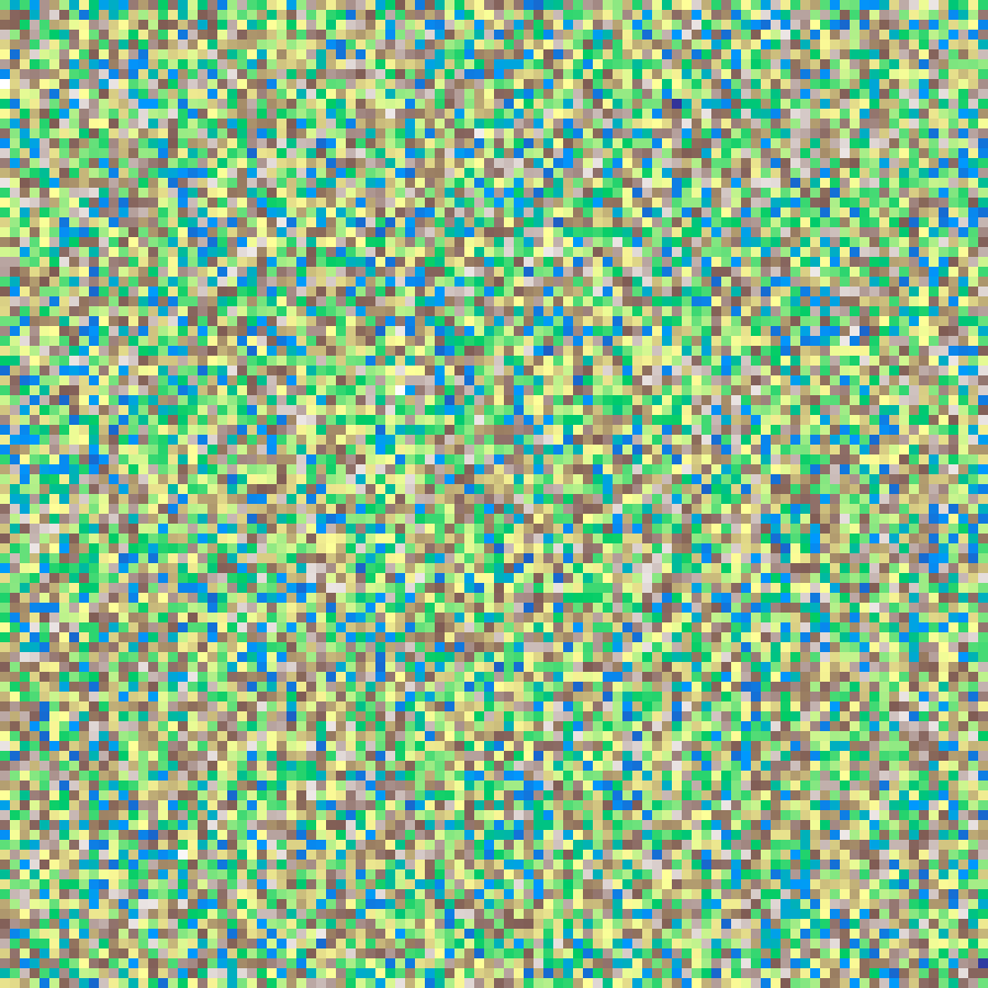
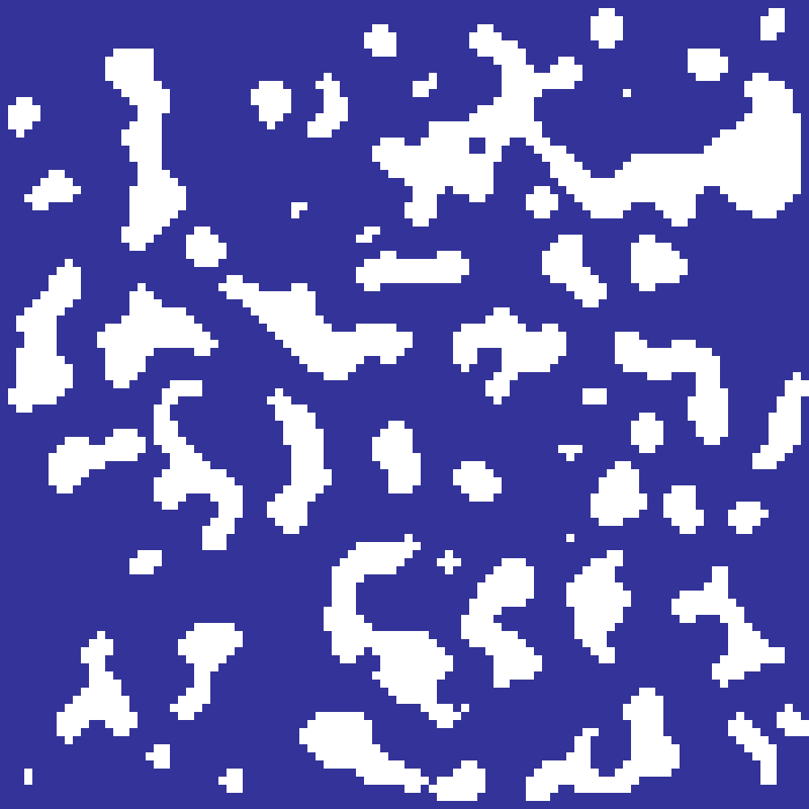
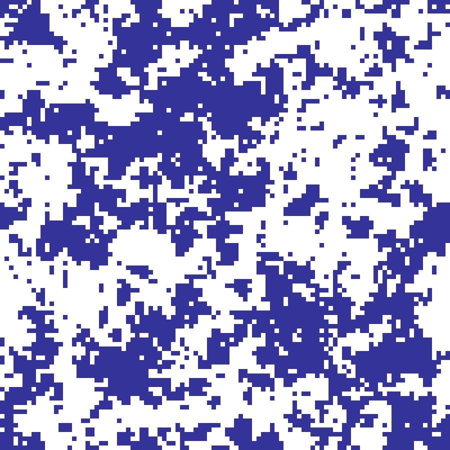
Percolation
percolation(rows: 100, cols: 100, p: 0.55, seed: 42)
Binary Bernoulli lattice where each cell is independently set to 1 with probability p, producing binary habitat maps. The critical percolation threshold for 4-connectivity is approximately 0.593.
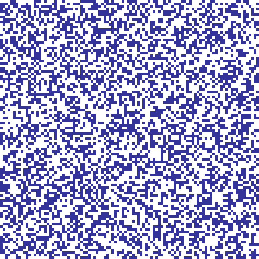
Source: Gardner et al. (1987)
Random Element
random_element(rows: 100, cols: 100, n: 5000, seed: 42)
Places n labelled seed cells at random positions, then fills all remaining cells with the value of the nearest seed using nearest-neighbour interpolation.
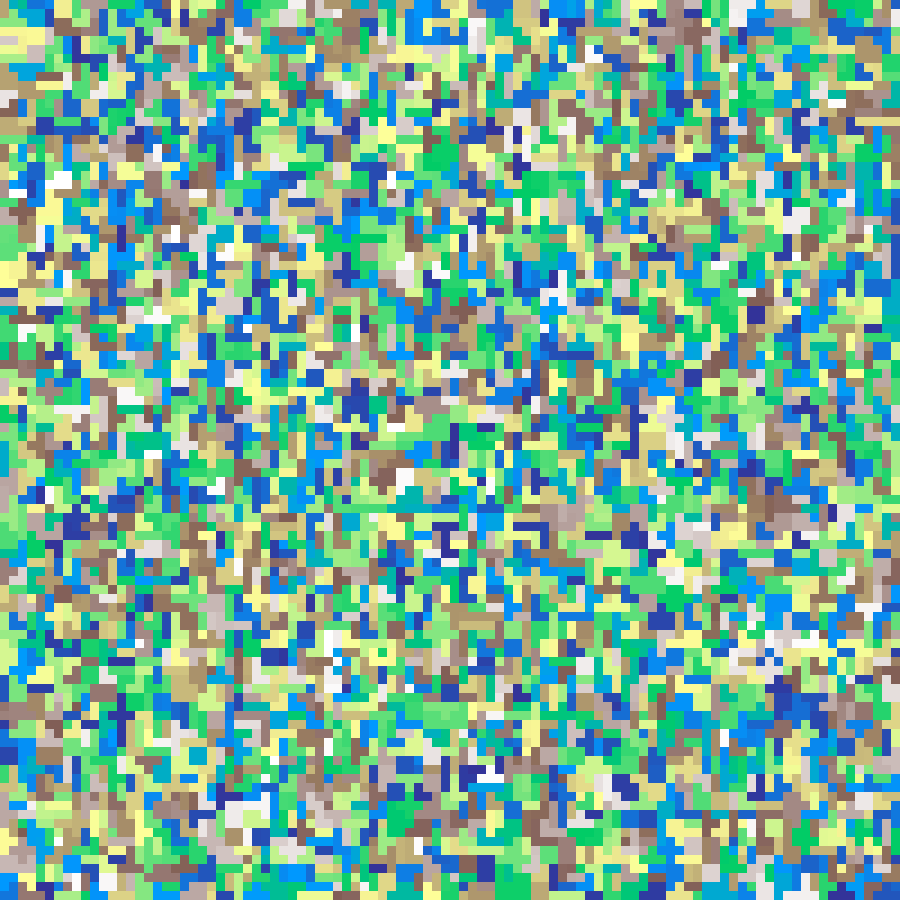
Source: Etherington, Holland & O'Sullivan (2015)
Poisson Disk
poisson_disk(rows: 100, cols: 100, min_dist: 5.0, seed: 42)
Uses Bridson's algorithm to place points such that no two are closer than min_dist. The resulting inhibition pattern has regular, even spacing compared to random point placement, modelling processes such as territorial behaviour or tree canopy competition.
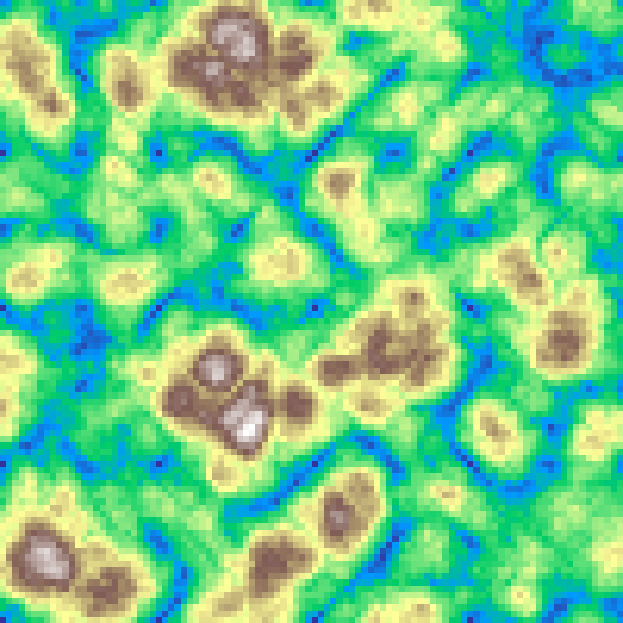
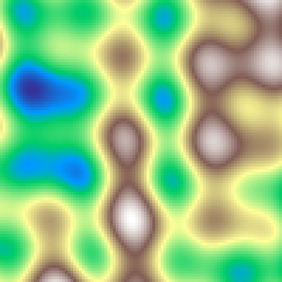
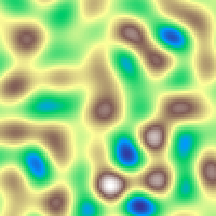
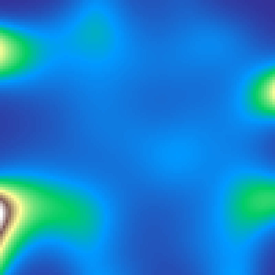
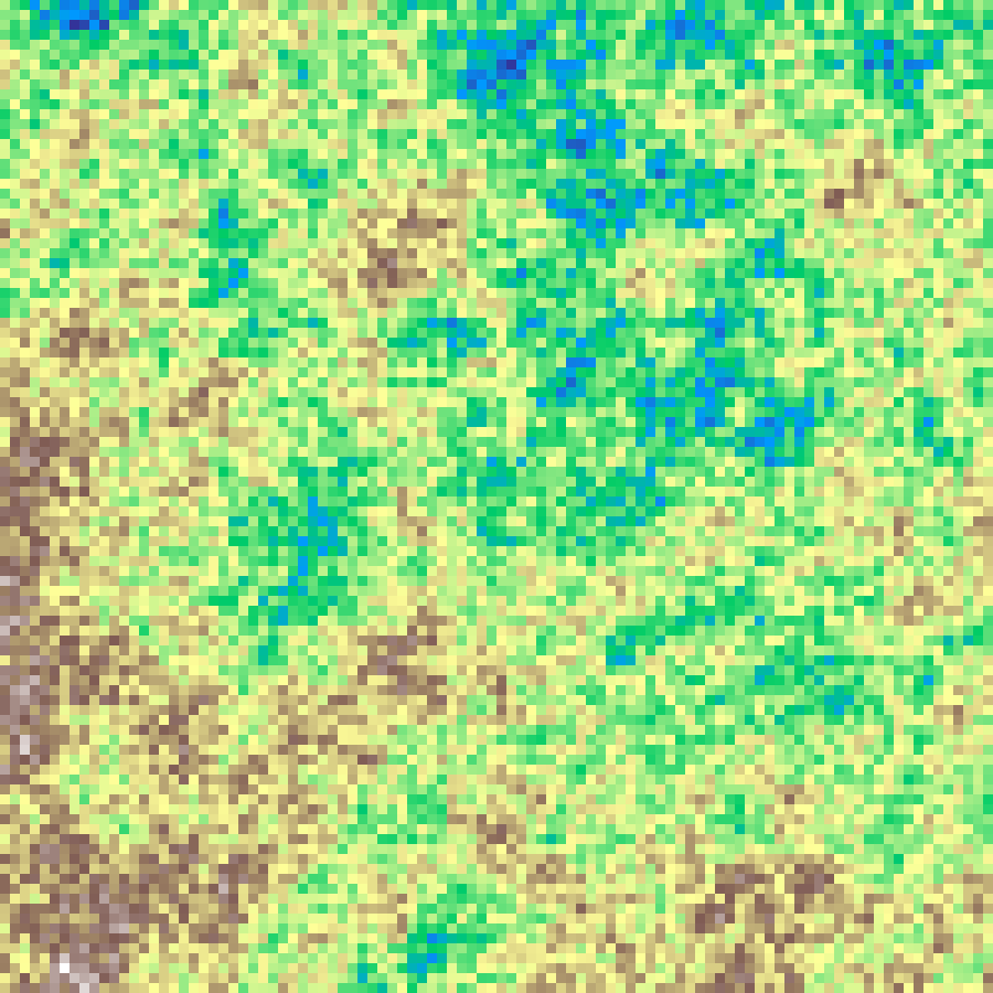
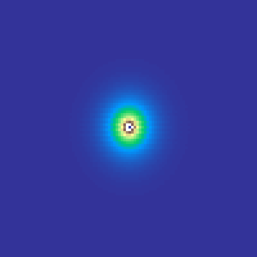
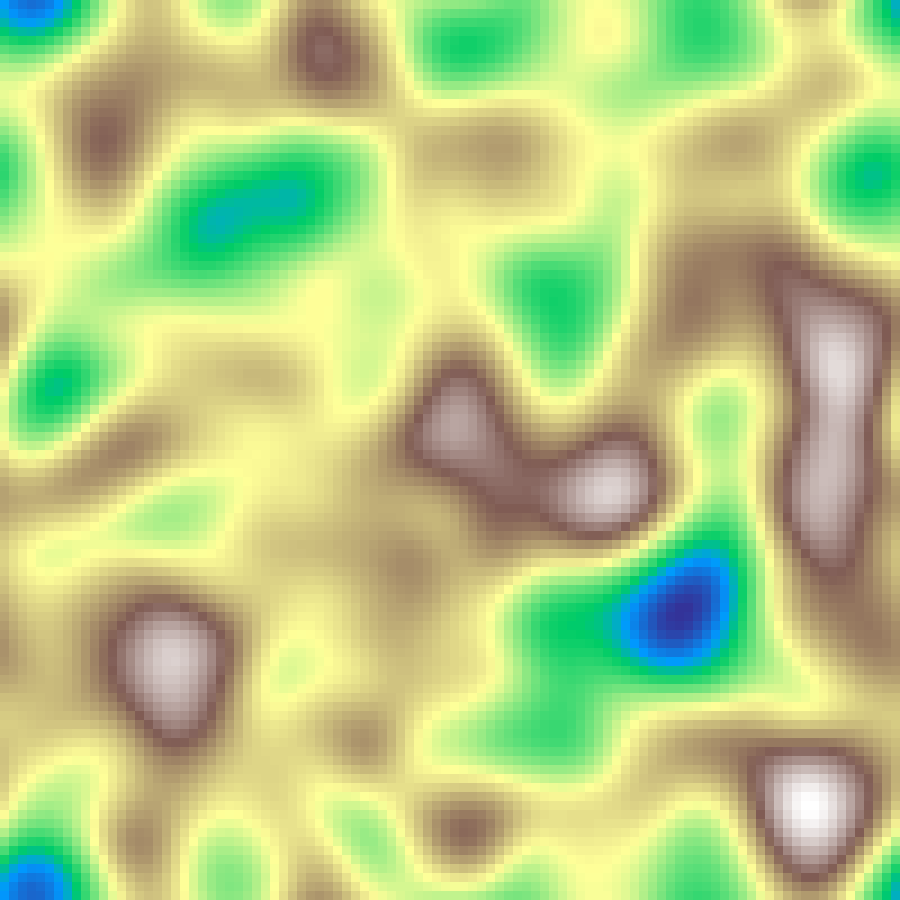
Gaussian Field
gaussian_field(rows: 100, cols: 100, sigma: 10.0, seed: 42)
White noise smoothed by a Gaussian blur kernel with standard deviation sigma, producing spatially correlated fields where patch size scales directly with sigma.
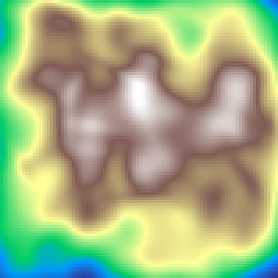
Gaussian Blobs
gaussian_blobs(rows: 100, cols: 100, n: 50, sigma: 5.0, seed: 42)
Places random Gaussian kernel centres and accumulates their contributions across the grid, then rescales to [0, 1]. Produces smooth blob-like elevation fields.
Random Cluster
random_cluster(rows: 100, cols: 100, n: 200, seed: 42)
Applies n random fault-line cuts across the grid, accumulating the field on each side, then rescales. Produces spatially clustered landscapes with the linear structural elements characteristic of geological fault patterns.
Source: Saura & Martínez-Millán (2000)
Rectangular Cluster
rectangular_cluster(rows: 100, cols: 100, n: 300, seed: 42)
Overlapping random axis-aligned rectangles accumulated and scaled, producing blocky clustered patches.
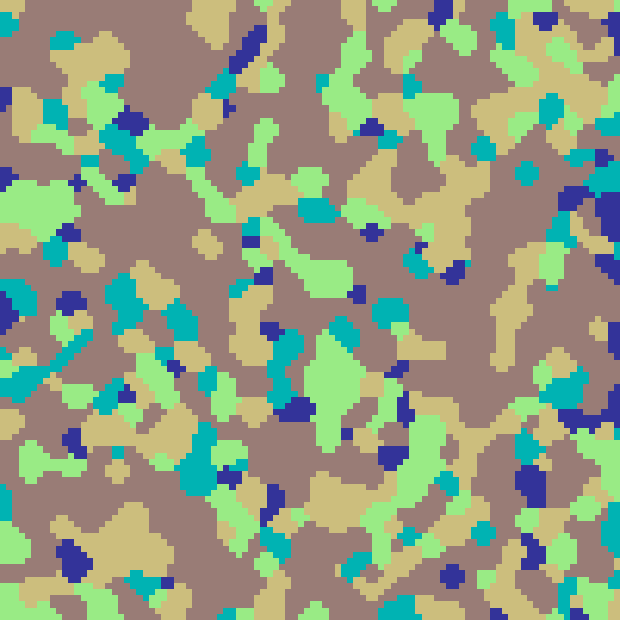
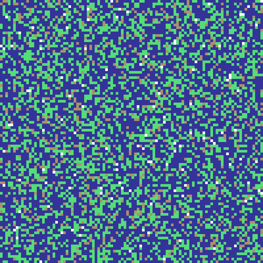
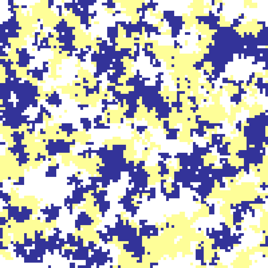
Neighbourhood Clustering
neighbourhood_clustering(rows: 100, cols: 100, k: 5, iterations: 10, seed: 42)
Initialises a grid with k random classes then repeatedly applies a majority-vote rule: each cell adopts the most common class in its 3×3 Moore neighbourhood. More iterations produce larger, smoother organic patches.
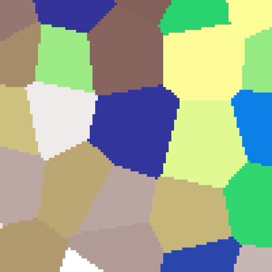
Mosaic
mosaic(rows: 100, cols: 100, n: 300, seed: 42)
Discrete Voronoi map where each region is a flat colour determined by its nearest seed point, producing a stained-glass or territory effect.
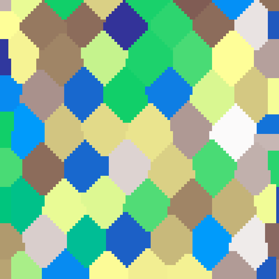
Hexagonal Voronoi
hexagonal_voronoi(rows: 100, cols: 100, n: 50, seed: 42)
Places seed points on a slightly jittered hexagonal lattice and uses nearest-neighbour BFS to fill each Voronoi cell with a random flat value, producing a regular honeycomb-like mosaic.
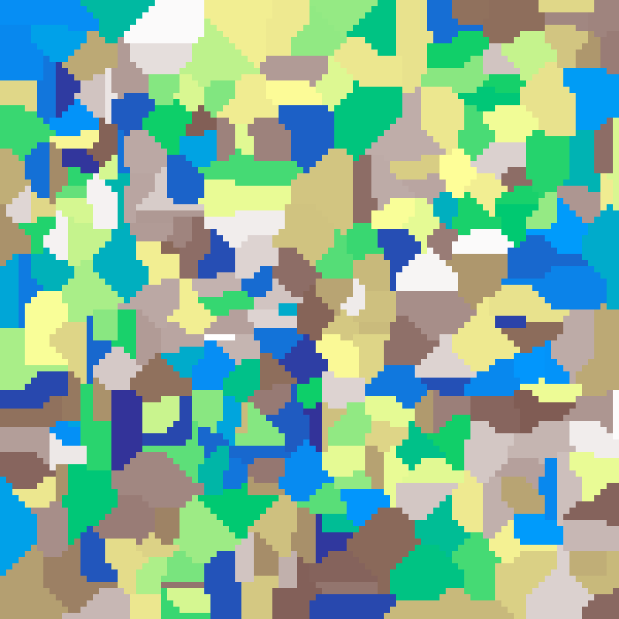
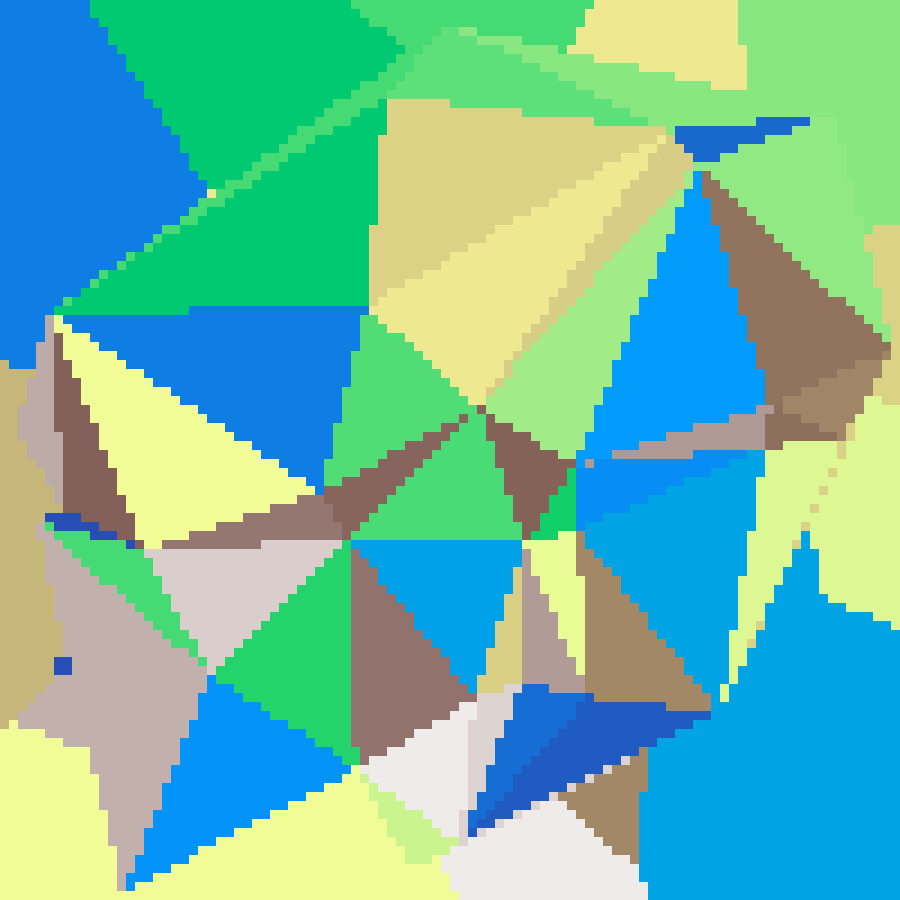
Triangular Tessellation
triangular_tessellation(rows: 100, cols: 100, n: 30, seed: 42)
Scatters n random points and computes their Delaunay triangulation via the Bowyer-Watson algorithm. Each triangle is assigned a uniform random value, producing a mosaic of flat-shaded triangles with straight edges.
Binary Space Partitioning
binary_space_partitioning(rows: 100, cols: 100, n: 200, seed: 42)
Hierarchical rectilinear partition: the largest rectangle is repeatedly split along its longest dimension until n leaf regions remain, each assigned a random value. Produces structured blocky landscapes.
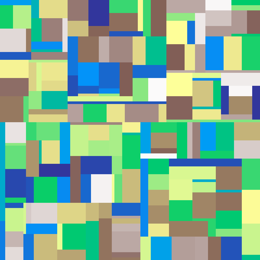
Source: Etherington, Morgan & O'Sullivan (2022)
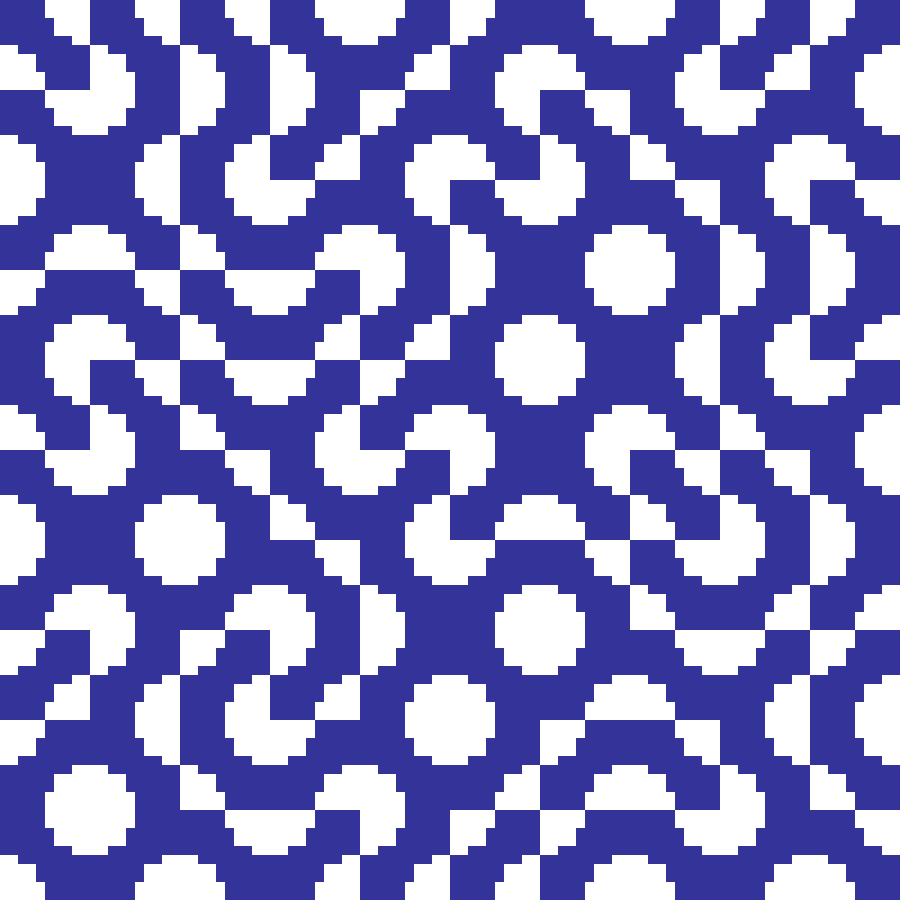
Truchet
truchet(rows: 100, cols: 100, n: 10, seed: 42)
Divides the grid into square macro-tiles of side n. Each tile is randomly assigned one of two orientations: quarter-circle arcs connecting either the top-left/bottom-right corners or the top-right/bottom-left corners. The interlocking curves produce flowing maze-like patterns.
Schelling
schelling(rows: 100, cols: 100, tolerance: 0.5, iterations: 50, seed: 42)
Schelling's model of residential segregation: cells of two types relocate to random empty slots whenever fewer than tolerance of their neighbours share their type. Even mild thresholds produce strong spatial segregation, generating sharp-edged binary cluster patterns.
Source: Schelling (1971)
Hill Grow
hill_grow(rows: 100, cols: 100, n: 20000, seed: 42)
Iteratively stamps a smooth convolution kernel at randomly selected cells, building up hill-like mounds. With runaway=True, taller cells attract more growth, causing hills to cluster into ridges.
Source: Etherington, Holland & O'Sullivan (2015)
Midpoint Displacement
midpoint_displacement(rows: 100, cols: 100, h: 0.8, seed: 42)
Recursive fractal terrain generation: grid midpoints are displaced by decreasing random amounts at each subdivision step, with h controlling the roughness (0 = rough, 1 = smooth).
Source: Fournier, Fussell & Carpenter (1982)
Fault Uplift
fault_uplift(rows: 100, cols: 100, n: 50, seed: 42)
Places n random fault lines across the grid and adds an exponential ridge of elevation along each one. Superimposing many ridges produces a crumpled, tectonically-inspired terrain with narrow elevated seams.
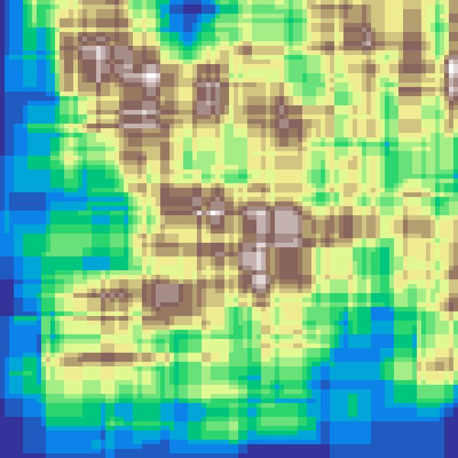
Hydraulic Erosion
hydraulic_erosion(rows: 100, cols: 100, n: 500, seed: 42)
Generates a random initial heightmap, then simulates n water droplets flowing downhill. Each droplet carries sediment, eroding steeper terrain and depositing on flatter areas. The result resembles naturally worn terrain with drainage channels, alluvial fans, and rounded ridges.
Thermal Erosion
thermal_erosion(rows: 100, cols: 100, n: 50, seed: 42)
Multi-octave Perlin heightmap eroded by repeated talus-slope diffusion. Each pass transfers material from steep cells to their lowest neighbour whenever the height difference exceeds the talus angle, smoothing cliffs while preserving gentle slopes.
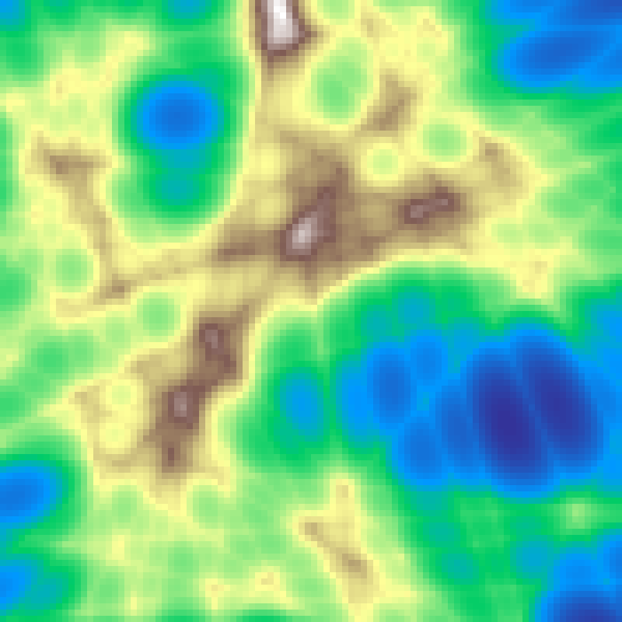
River Network
river_network(rows: 100, cols: 100, seed: 42)
Generates a fractal Brownian terrain, computes D8 steepest-descent flow directions, then accumulates upstream drainage area. Log-scaling the flow accumulation reveals branching river networks with realistic headwater-to-trunk gradients.
Cellular Automaton
cellular_automaton(rows: 100, cols: 100, p: 0.45, iterations: 5, seed: 42)
Random binary grid evolved by Conway-style birth/survival rules: a dead cell is born if it has at least birth_threshold live neighbours; a live cell survives if it has at least survival_threshold. Produces cave-like binary landscapes.
Game of Life
game_of_life(rows: 100, cols: 100, iterations: 200, seed: 42)
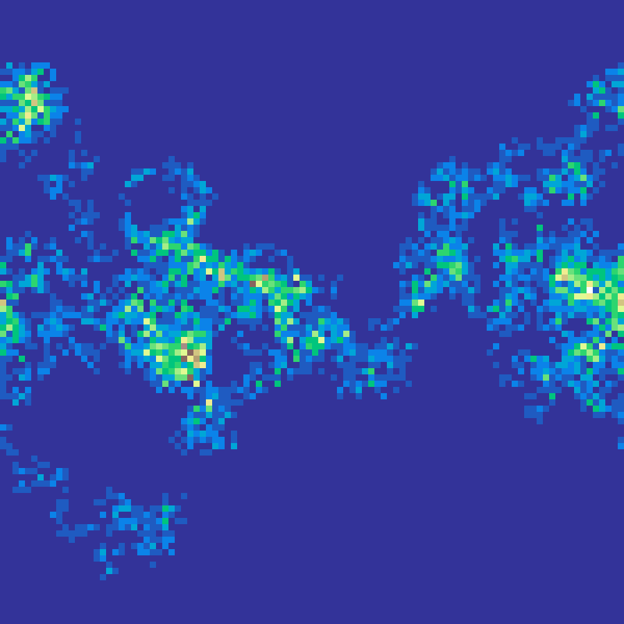
Conway's B3/S23 cellular automaton run on a random initial state. Cells are born with exactly 3 live neighbours and survive with 2 or 3; all other cells die. The output is the visit-density: the fraction of generations each cell spent alive, revealing long-lived stable structures, oscillators, and glider paths.
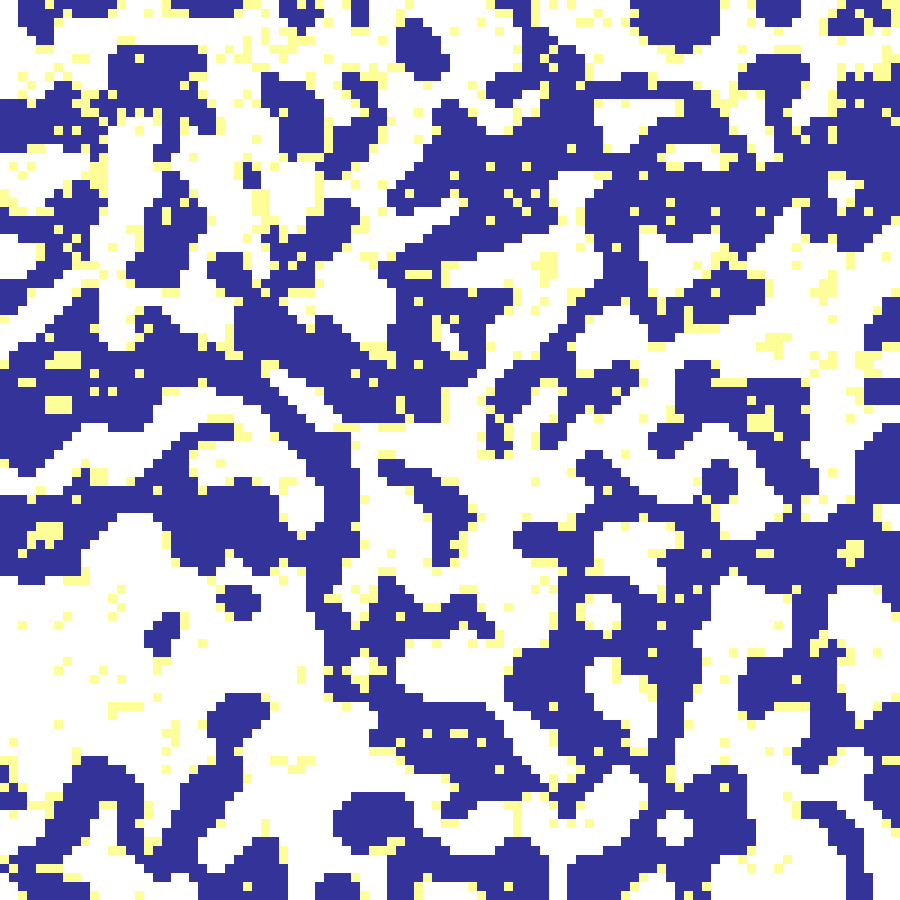
Ising Model
ising_model(rows: 100, cols: 100, beta: 0.4, iterations: 1000, seed: 42)
Simulates a 2D Ising spin lattice via Glauber dynamics. Near the critical inverse temperature (β ≈ 0.44) the model produces scale-free, patchy binary patterns reminiscent of habitat mosaics.
Sandpile
sandpile(rows: 100, cols: 100, n: 5000, seed: 42)
Bak-Tang-Wiesenfeld sandpile model: n grains are dropped at random cells; any cell accumulating 4 or more grains topples, distributing one grain to each of its four neighbours. The resulting grain-count map reveals self-similar avalanche structure characteristic of self-organized criticality.
Source: Bak, Tang & Wiesenfeld (1987)
Forest Fire
forest_fire(rows: 100, cols: 100, p_tree: 0.02, p_lightning: 0.001, iterations: 500, seed: 42)
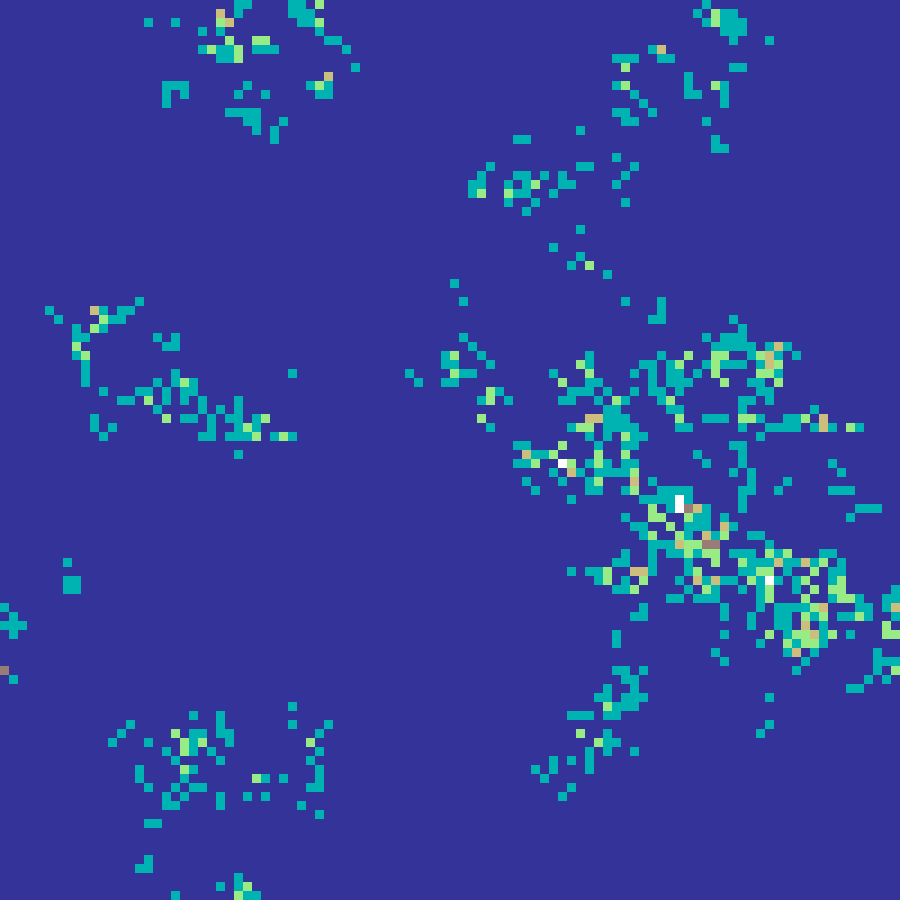
Drossel-Schwabl forest fire cellular automaton: empty cells grow trees with probability p_tree; trees ignite from lightning with probability p_lightning and spread to neighbouring trees. The cumulative burn count, scaled to [0, 1], captures spatial fire-scar patterns.
Crystal Growth
crystal_growth(rows: 100, cols: 100, iterations: 300, seed: 42)
Reiter's (1996) hexagonal cellular automaton model of snowflake growth. A single frozen seed at the centre absorbs water vapour from receptive cells (those adjacent to the crystal), which freeze when their accumulated level reaches 1. The result is a six-fold symmetric crystal with intricate branching arms.
Source: Reiter (1996)
Cahn-Hilliard
cahn_hilliard(rows: 100, cols: 100, iterations: 2000, seed: 42)
Numerically integrates the Cahn-Hilliard PDE for spinodal decomposition: ∂u/∂t = ∇²(u³ - u - ε²∇²u). Starting from small random perturbations, a binary mixture spontaneously phase-separates into smooth, rounded domains that coarsen over time.
Eden Growth
eden_growth(rows: 100, cols: 100, n: 2000, seed: 42)
Compact cluster grown from the grid centre by randomly selecting a boundary cell at each step. Produces irregular blob shapes with fractal perimeters.

Diffusion-Limited Aggregation
diffusion_limited_aggregation(rows: 100, cols: 100, n: 2000, seed: 42)
Random-walking particles released from a spawn ring stick when adjacent to the growing cluster, producing intricate branching fractal structures.
Invasion Percolation
invasion_percolation(rows: 100, cols: 100, n: 2000, seed: 42)
Grows a cluster from the grid centre by always invading the boundary cell with the lowest random weight, producing fractal-like connected binary patches.
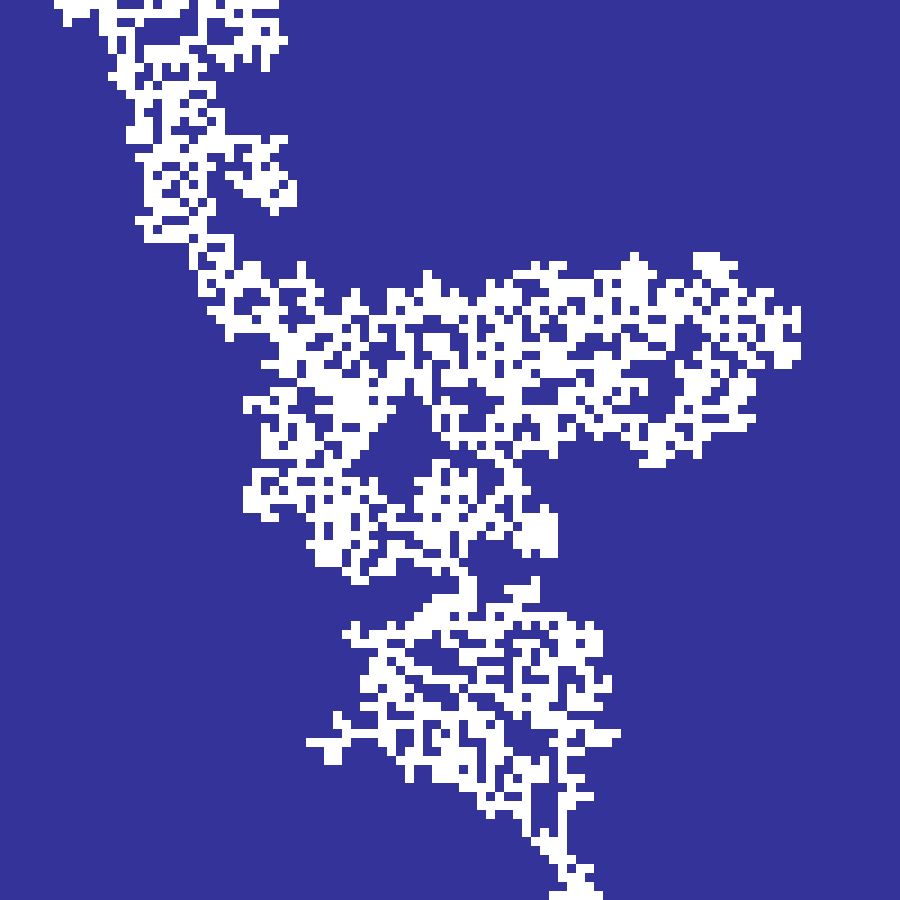
Physarum
physarum(rows: 100, cols: 100, n: 1000, iterations: 300, seed: 42)
Agent-based simulation of Physarum polycephalum (slime mould). Agents sense a chemical trail at ±45° ahead and steer toward the strongest signal, then deposit trail at their new position. Trail diffuses and decays at each step. The emergent network of reinforced paths resembles efficient transport networks.
Source: Jones (2010)
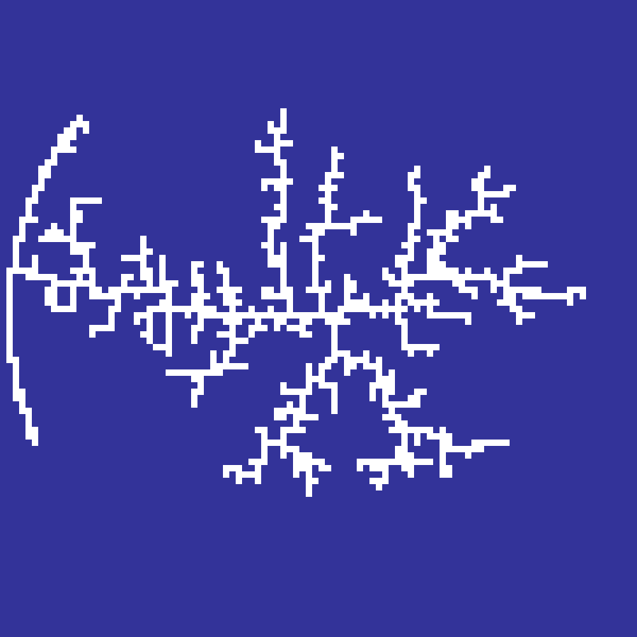
Space Colonization
space_colonization(rows: 100, cols: 100, n: 200, seed: 42)
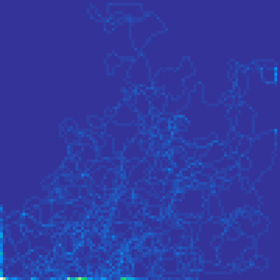
Auxin-based vascular branching network (Runions et al. 2005). Random auxin attractors in the upper portion of the grid draw nearby network nodes toward them; attractors within the kill distance are consumed. The result is a hierarchical branching tree resembling leaf venation or river tributaries.

Source: Runions et al. (2005)
Brownian Motion
brownian_motion(rows: 100, cols: 100, n: 5000, seed: 42)
Simulates n steps of a 2D Brownian random walk on a toroidal grid and accumulates visit counts, producing a visit-density map with dense hotspots along the walker's path.
Levy Flight
levy_flight(rows: 100, cols: 100, n: 1000, seed: 42)
Simulates a Levy flight: a random walk where step lengths follow a power-law (heavy-tailed) distribution. The resulting visit-density map has clustered hotspots with occasional long-range jumps, modelling dispersal or foraging patterns.
Correlated Walk
correlated_walk(rows: 100, cols: 100, n: 5000, kappa: 2.0, seed: 42)
A random walk where each step direction is drawn from a wrapped normal distribution centred on the previous heading. Higher kappa values produce straighter, more directional trajectories; kappa = 0 reduces to isotropic Brownian motion. The visit-density map models correlated animal movement or dispersal paths.
Substrate
substrate(rows: 100, cols: 100, n: 10, seed: 42)
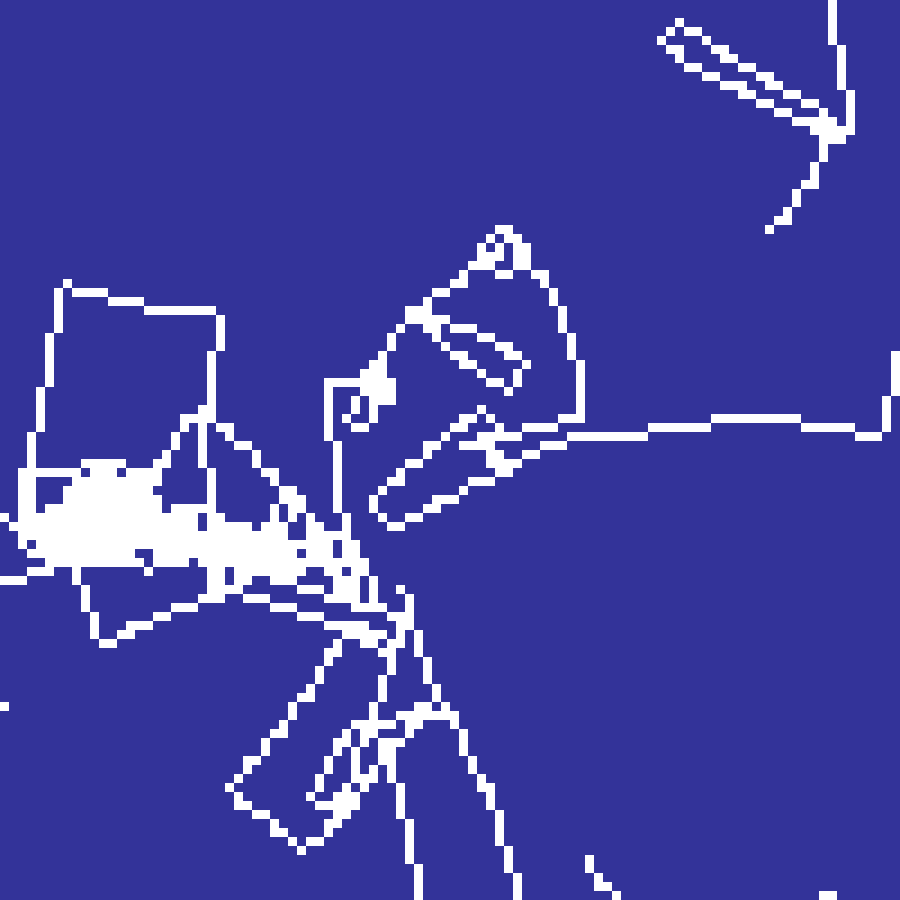
Jared Tarbell's crack propagation algorithm. Cracks originate from random seed points and propagate with a small Gaussian angular deviation each step. When a crack meets an existing crack it deflects perpendicularly, producing an organic network of intersecting fractures reminiscent of dried mud or cracked glaze.
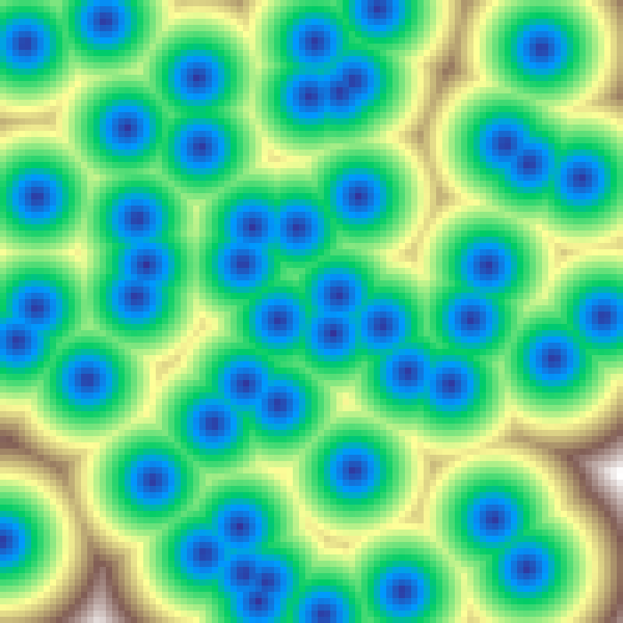
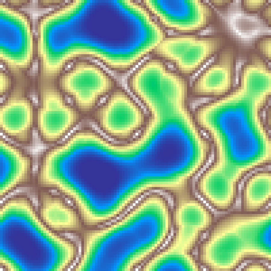
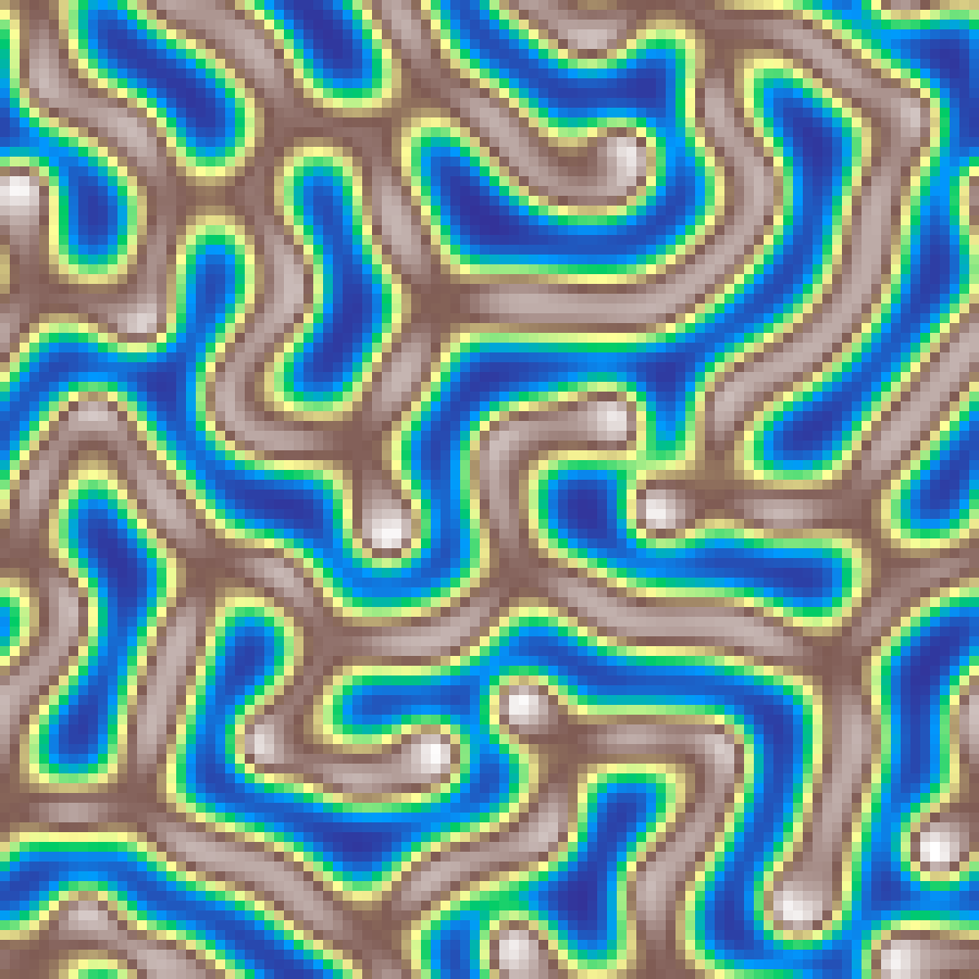
Reaction-Diffusion
reaction_diffusion(rows: 100, cols: 100, iterations: 1000, feed: 0.055, kill: 0.062, seed: 42)
Gray-Scott reaction-diffusion model where two chemicals (A and B) diffuse and react across the grid. Different feed/kill combinations produce spots, stripes, labyrinths, and other Turing-pattern morphologies.
Excitable Media
excitable_media(rows: 100, cols: 100, iterations: 150, seed: 42)
Greenberg-Hastings excitable media model. Each cell cycles through resting, excited, and refractory states. A resting cell becomes excited if any cardinal neighbour is excited; excited cells enter a refractory chain before returning to rest. Random initial states seed broken wave fronts that self-organise into propagating spiral waves and target patterns.
Predator-Prey
predator_prey(rows: 100, cols: 100, iterations: 500, seed: 42)
Spatial Lotka-Volterra PDE with diffusion. Two fields, prey (u) and predators (v), interact via classic predation kinetics while diffusing across the grid. Initialised near the coexistence equilibrium with small noise, the system self-organises into travelling waves and spiral patterns.
SIR Epidemic
sir_epidemic(rows: 100, cols: 100, beta: 0.3, gamma: 0.1, iterations: 200, seed: 42)
Spatial SIR reaction-diffusion model. Susceptible (S), infected (I), and recovered (R) compartments evolve via a PDE with diffusion and mass-action infection kinetics. The output is the recovered field, showing which regions were swept by the epidemic wavefront.
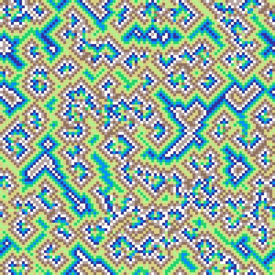
Rock-Paper-Scissors
rock_paper_scissors(rows: 100, cols: 100, iterations: 200, seed: 42)
Spatial cyclic dominance model with three competing species (0, 1, 2). Each generation performs rows × cols Monte-Carlo trials: a random cell is selected along with one random neighbour; if the neighbour carries the predator state (state + 1) % 3, the cell is consumed. Asynchronous updates allow domains to coarsen and rotate into the characteristic spiral waves of cyclic competition.
Usage
nlmrs is available as a Rust crate or as a CLI tool. Language bindings are also provided for Python, R, Julia, WASM, and C.
cargo add nlmrs
use nlmrs;

fn main() {
    let grid = nlmrs::midpoint_displacement(100, 100, 1.0, seed: Some(42));
    println!("{:?}", grid.data);
}
Export
The export module provides functions to save a grid to disk.
use nlmrs::{midpoint_displacement, export};

fn main() {
    let grid = midpoint_displacement(rows: 100, cols: 100, h: 0.8, Some(42));

    export::write_to_png(&grid, "terrain.png").unwrap();
    export::write_to_png_grayscale(&grid, "terrain_gray.png").unwrap();
    export::write_to_tiff(&grid, "terrain.tif").unwrap();
    export::write_to_csv(&grid, "terrain.csv").unwrap();
    export::write_to_json(&grid, "terrain.json").unwrap();
    export::write_to_ascii_grid(&grid, "terrain.asc").unwrap();
}
CLI
A command-line binary is included. Output format is inferred from the file extension (.png, .csv, .json, .tif, .asc).
cargo install nlmrs

nlmrs midpoint-displacement 200 200 --h 0.8 --seed 42 --output terrain.png
nlmrs fbm 300 300 --scale 6.0 --octaves 8 --seed 99 --output landscape.png
nlmrs hill-grow 200 200 --n 20000 --runaway --output hills.csv
nlmrs perlin 500 500 --scale 4.0 --grayscale --output noise.png

nlmrs --help   # list all subcommands and options
Grid operations
The operation module exposes combinators for building composite NLMs:
use nlmrs::{midpoint_displacement, planar_gradient, operation};

fn main() {
    let mut terrain = midpoint_displacement(100, 100, 0.8, Some(1));
    let gradient   = planar_gradient(100, 100, Some(90.), Some(2));

    operation::multiply(&mut terrain, &gradient);
    operation::scale(&mut terrain);
}
Available operations: add, add_value, multiply, multiply_value, invert, abs, scale, min, max, min_and_max, classify, threshold.
Python bindings
nlmrs is available as a Python package. Every function returns a 2D numpy array.
Install
pip install nlmrs
Or build from source (requires Rust and maturin):
maturin develop --features python # editable install into the active venv
Usage
import nlmrs
import matplotlib.pyplot as plt

# All functions accept an optional seed for reproducible output.
grid = nlmrs.midpoint_displacement(100, 100, h=0.8, seed=42)  # numpy array (100, 100)

plt.imshow(grid, cmap="terrain")
plt.axis("off")
plt.show()
Post-processing functions are also available:
grid = nlmrs.fbm_noise(100, 100, scale=4.0)
nlmrs.classify(grid, n=5)    # quantise into n equal-width classes
nlmrs.threshold(grid, t=0.5) # binarise at threshold t
R bindings
nlmrs is available as an R package via the extendr framework. Every function returns a numeric matrix.
Install
# Install from source (requires Rust)
remotes::install_github("tom-draper/nlmrs", subdir = "bindings/r")
Usage
library(nlmrs)

# All functions accept an optional integer seed.
m <- nlm_midpoint_displacement(100, 100, h = 0.8, seed = 42L)
image(m, col = terrain.colors(256))
Julia bindings
nlmrs is available as a Julia package. Every function returns a Matrix{Float64}.
Install
# Requires Rust (https://rustup.rs) - builds the C library automatically.
import Pkg
Pkg.add(url="https://github.com/tom-draper/nlmrs", subdir="bindings/julia")
Usage
using nlmrs

# All functions accept an optional seed keyword for reproducible output.
m = midpoint_displacement(100, 100, h=0.8, seed=42)  # Matrix{Float64} (100, 100)
C bindings
nlmrs exposes a C-compatible shared/static library, making it usable from any language with C FFI support (C++, Go, MATLAB, Fortran, etc.).
Build
cd bindings/c
cargo build --release
# → ../../target/release/libnlmrs_c.so   (Linux shared)
# → ../../target/release/libnlmrs_c.a    (Linux static)
# → include/nlmrs.h                       (generated header)
Usage
#include "nlmrs.h"
#include <stdio.h>

int main(void) {
    uint64_t seed = 42;

    // Generate a 200×200 midpoint displacement grid.
    NlmGrid grid = nlmrs_midpoint_displacement(200, 200, 0.8, &seed);

    printf("rows=%zu cols=%zu\n", grid.rows, grid.cols);

    // Access row-major data: value at (r, c) = grid.data[r * grid.cols + c]
    printf("value at (0,0): %f\n", grid.data[0]);

    nlmrs_free(grid);   // release Rust-owned memory
    return 0;
}
Compile and link against the shared library:
gcc example.c -I bindings/c/include -L target/release -lnlmrs_c -o example
Optional parameters
Seeds and optional floats (e.g. gradient direction) are passed as pointers. Pass NULL to use the default (random seed / random direction):
// Random seed
NlmGrid g1 = nlmrs_perlin_noise(200, 200, 4.0, NULL);

// Fixed direction, random seed
double dir = 45.0;
NlmGrid g2 = nlmrs_planar_gradient(200, 200, &dir, NULL);

nlmrs_free(g1);
nlmrs_free(g2);
The header include/nlmrs.h is generated automatically by cbindgen during the build.
WASM bindings
nlmrs can run in the browser or Node.js via WebAssembly.
Build
cd bindings/wasm
wasm-pack build --target web
Usage
import init, * as nlmrs from "./pkg/nlmrs_wasm.js";

await init();

const grid = nlmrs.midpoint_displacement(100, 100, 0.8, 42);
console.log(grid.rows, grid.cols);   // 100 100

// Flat Float64Array in row-major order
const flat = grid.data;
const value = flat[r * grid.cols + c];

grid.free();  // release Rust memory
Seeds are passed as plain integers. Omit the seed argument for random output.
Contributions
Contributions, issues and feature requests are welcome.
- Fork it (https://github.com/tom-draper/nlmrs)
- Create your feature branch (
git checkout -b my-new-feature) - Commit your changes (`git commit -am 'Add some feature')
- Push to the branch (
git push origin my-new-feature) - Create a new Pull Request
Project details
Verified details
These details have been verified by PyPIProject links
GitHub Statistics
Maintainers


Download files
Download the file for your platform. If you're not sure which to choose, learn more about installing packages.
Source Distribution
Built Distributions
Filter files by name, interpreter, ABI, and platform.
If you're not sure about the file name format, learn more about wheel file names.
Copy a direct link to the current filters
File details
Details for the file nlmrs-0.2.4.tar.gz.
File metadata
- Download URL: nlmrs-0.2.4.tar.gz
- Upload date:
- Size: 2.0 MB
- Tags: Source
- Uploaded using Trusted Publishing? Yes
- Uploaded via: maturin/1.12.6
File hashes
| Algorithm | Hash digest | |
|---|---|---|
| SHA256 |
8a0bd73db31f6b257e0fe1315ddc0d32ecc4d0407cf4adf14b0fad5af8745c53
|
|
| MD5 |
ad6c99e9b9878b62144a657e3a0a2e79
|
|
| BLAKE2b-256 |
04e5877c92265f61238f2b075fe220094f1ad0d4cf7ede1ab611eb339ed5495f
|
File details
Details for the file nlmrs-0.2.4-pp310-pypy310_pp73-manylinux_2_17_aarch64.manylinux2014_aarch64.whl.
File metadata
- Download URL: nlmrs-0.2.4-pp310-pypy310_pp73-manylinux_2_17_aarch64.manylinux2014_aarch64.whl
- Upload date:
- Size: 825.3 kB
- Tags: PyPy, manylinux: glibc 2.17+ ARM64
- Uploaded using Trusted Publishing? Yes
- Uploaded via: maturin/1.12.6
File hashes
| Algorithm | Hash digest | |
|---|---|---|
| SHA256 |
3987f53b04d9fe495faa638743c56ecb44288a095f9fee98ad4d9fb56c6f2e0a
|
|
| MD5 |
f9f2f41446b992ac610f706ba55bc063
|
|
| BLAKE2b-256 |
c5daaf0268ed3fd900591e594547c011d23054eb10e54a849fa990650c0b236d
|
File details
Details for the file nlmrs-0.2.4-pp39-pypy39_pp73-manylinux_2_17_aarch64.manylinux2014_aarch64.whl.
File metadata
- Download URL: nlmrs-0.2.4-pp39-pypy39_pp73-manylinux_2_17_aarch64.manylinux2014_aarch64.whl
- Upload date:
- Size: 825.3 kB
- Tags: PyPy, manylinux: glibc 2.17+ ARM64
- Uploaded using Trusted Publishing? Yes
- Uploaded via: maturin/1.12.6
File hashes
| Algorithm | Hash digest | |
|---|---|---|
| SHA256 |
849750b587339b47b87f56fb6fd267e46762a1a147a33e77f10b919612cb8c58
|
|
| MD5 |
ddb492f36fe91a4624314a72e95681f5
|
|
| BLAKE2b-256 |
ec5e37020d6a2802033cc46af55724cb1e3733ecfb6786b63c61accaea58bca4
|
File details
Details for the file nlmrs-0.2.4-pp38-pypy38_pp73-manylinux_2_17_aarch64.manylinux2014_aarch64.whl.
File metadata
- Download URL: nlmrs-0.2.4-pp38-pypy38_pp73-manylinux_2_17_aarch64.manylinux2014_aarch64.whl
- Upload date:
- Size: 825.7 kB
- Tags: PyPy, manylinux: glibc 2.17+ ARM64
- Uploaded using Trusted Publishing? Yes
- Uploaded via: maturin/1.12.6
File hashes
| Algorithm | Hash digest | |
|---|---|---|
| SHA256 |
e1a8b65cb46285eccc16634f461cddc413d6ba34ccb11cd0840a2e277b375055
|
|
| MD5 |
323ed0b1860a4d87f7f8da67771aaee4
|
|
| BLAKE2b-256 |
292dd559d572492663e93a6cc1122ec9b8bba1858af38fb820bbe8336eb31093
|
File details
Details for the file nlmrs-0.2.4-pp37-pypy37_pp73-manylinux_2_17_aarch64.manylinux2014_aarch64.whl.
File metadata
- Download URL: nlmrs-0.2.4-pp37-pypy37_pp73-manylinux_2_17_aarch64.manylinux2014_aarch64.whl
- Upload date:
- Size: 827.5 kB
- Tags: PyPy, manylinux: glibc 2.17+ ARM64
- Uploaded using Trusted Publishing? Yes
- Uploaded via: maturin/1.12.6
File hashes
| Algorithm | Hash digest | |
|---|---|---|
| SHA256 |
e4d576571fc9a0c783e7fa47d944a6df6bfd06b1da4b3421adf2d036bc6fd724
|
|
| MD5 |
95235f435208ce38a1ba55eb771888bb
|
|
| BLAKE2b-256 |
bea8943257223c5555d911134fa04934ae9dce91fa36cc9689228be82c0285e2
|
File details
Details for the file nlmrs-0.2.4-cp38-abi3-win_amd64.whl.
File metadata
- Download URL: nlmrs-0.2.4-cp38-abi3-win_amd64.whl
- Upload date:
- Size: 745.1 kB
- Tags: CPython 3.8+, Windows x86-64
- Uploaded using Trusted Publishing? Yes
- Uploaded via: maturin/1.12.6
File hashes
| Algorithm | Hash digest | |
|---|---|---|
| SHA256 |
9e262e795263b04639280c9ba4ed0e79561511585708fd3d81cb6433247e9c28
|
|
| MD5 |
837c4b597bad3ca9e0d0a8455a0914e2
|
|
| BLAKE2b-256 |
298b5eb53c6f959b70d3f7b190a291c037a612dd8bf316b63f75a072eaf94e23
|
File details
Details for the file nlmrs-0.2.4-cp38-abi3-manylinux_2_17_x86_64.manylinux2014_x86_64.whl.
File metadata
- Download URL: nlmrs-0.2.4-cp38-abi3-manylinux_2_17_x86_64.manylinux2014_x86_64.whl
- Upload date:
- Size: 946.6 kB
- Tags: CPython 3.8+, manylinux: glibc 2.17+ x86-64
- Uploaded using Trusted Publishing? Yes
- Uploaded via: maturin/1.12.6
File hashes
| Algorithm | Hash digest | |
|---|---|---|
| SHA256 |
3329bae74ddbf4bf59d3820579fa368d4171dd4b7cf971fed061bca3da5edb65
|
|
| MD5 |
e0674a82203ae51fd759e9f1753460cc
|
|
| BLAKE2b-256 |
442dffbb8fa72a0729a3962b1af1449c07fe00cf65e3e87a89fd4e22bb76b35c
|
File details
Details for the file nlmrs-0.2.4-cp38-abi3-manylinux_2_17_aarch64.manylinux2014_aarch64.whl.
File metadata
- Download URL: nlmrs-0.2.4-cp38-abi3-manylinux_2_17_aarch64.manylinux2014_aarch64.whl
- Upload date:
- Size: 829.9 kB
- Tags: CPython 3.8+, manylinux: glibc 2.17+ ARM64
- Uploaded using Trusted Publishing? Yes
- Uploaded via: maturin/1.12.6
File hashes
| Algorithm | Hash digest | |
|---|---|---|
| SHA256 |
5bcf6468bc5839dcf9a371356af6a4bd9d0504aa7c614df7116a0ccdbcce5307
|
|
| MD5 |
4b2e8c17b1e96a5ed6da7017c4d3f48f
|
|
| BLAKE2b-256 |
aa7955532080902377a033048835386aec3ac7abd5f6ec57140d64de1cb7d0ef
|
File details
Details for the file nlmrs-0.2.4-cp38-abi3-macosx_11_0_arm64.whl.
File metadata
- Download URL: nlmrs-0.2.4-cp38-abi3-macosx_11_0_arm64.whl
- Upload date:
- Size: 750.3 kB
- Tags: CPython 3.8+, macOS 11.0+ ARM64
- Uploaded using Trusted Publishing? Yes
- Uploaded via: maturin/1.12.6
File hashes
| Algorithm | Hash digest | |
|---|---|---|
| SHA256 |
9a91af5163c5ccb27fef97860ac8f7a5c8e580f7d638eec151115c7fa2720a28
|
|
| MD5 |
535cb1e133d84ac2835ebcbc490fddde
|
|
| BLAKE2b-256 |
79e3a4b9680f2ecead6ef26e4614655df215ecbd21b59385227576c1893a999d
|
File details
Details for the file nlmrs-0.2.4-cp38-abi3-macosx_10_12_x86_64.whl.
File metadata
- Download URL: nlmrs-0.2.4-cp38-abi3-macosx_10_12_x86_64.whl
- Upload date:
- Size: 854.7 kB
- Tags: CPython 3.8+, macOS 10.12+ x86-64
- Uploaded using Trusted Publishing? Yes
- Uploaded via: maturin/1.12.6
File hashes
| Algorithm | Hash digest | |
|---|---|---|
| SHA256 |
e159b977013ebab0c5104f7cd4ada4129ad6b9abab61c35584cdfa9f80244b69
|
|
| MD5 |
ed7bd0ffe9f7e2b821248ea58f88e85f
|
|
| BLAKE2b-256 |
d71714c468ca365e4f7327a7ab635205cad56fc788fdeedfc637ab179c3d1a75
|


