
noisestate
Equilibrium solver for linear-quadratic-Gaussian games with private information. Describe the states, what each agent observes, and what each agent wants to minimise in YAML or Python. Solve for causal linear strategies, then inspect each agent's cost and how states and actions respond to shocks.
The solver returns both responses to the primitive shocks (the noise-state representation) and strategies on each agent's own signal history. It also decomposes the first-order conditions into the instantaneous part, the physical continuation and the information wedge.
The framework follows the dissertation Noise-State Calculus for Dynamic Games with Strategic Information (Babichenko, 2026). Agents influence a shared state through their controls and observe noisy signals of states and other agents' actions. Each minimises a discounted or average quadratic loss.
Can this solve my problem?
Use noisestate for games with linear state dynamics and observations, Brownian noise, and quadratic running objectives. It solves for causal linear strategies: each agent's action depends on its own observations up to the current time. Models can have a finite horizon, a stationary regime, or a transition between regimes, with supported observation and action delays.
Hard control constraints such as D >= 0, nonlinear dynamics, and terminal penalties such as
X(T)^2 are outside the model grammar. The solution is sought within the causal linear strategy
class; see limits for the assumptions and restrictions of each engine.
Install
From the repository's root directory:
pip install ".[plot]" # from a checkout of this repository; [plot] adds matplotlib
Python >= 3.10. Dependencies: numpy >= 1.24, scipy >= 1.12, pyyaml; matplotlib for the figures, which
the walkthrough below draws. MIT licence. The shipped model files install with the package, so
ns.example(...) works from a plain install; the reference data (tests/refs/) lives in the
repository only.
A first game, start to finish
This walkthrough uses ch1_two_player_finite, the Chapter 1 tracking game, to introduce the model
format, solve a game, interpret the result, and change a parameter.
The game
Two players share one state and each watches it through their own noisy signal. Both want the state at zero, and both pay for the effort of pushing it there:
dX  = (D1 + D2) dt + sigma dW0            one state, moved by both players and by a common shock
dYi = sqrt(pi) X dt + dWi                 player i sees X through its own noise; pi is its precision
player i minimises  E int_0^T (X^2 + ri Di^2) dt
The state starts at the known value X(0) = 0. The Brownian channels W0, W1, and W2 are
independent. Player i observes only its own signal history Yi up to the current time; it does
not directly observe X, the shocks, or the other player's signal. The common shock moves the
shared state; "common" does not mean that the players see it directly.
This is the same model as a file (an omitted state initial defaults to zero here):
name: ch1_two_player_finite
params: {p1: 3.0, p2: 3.0, r1: 0.1, r2: 0.1, sigma: 1.0}
channels: [w0, w1, w2]                                   # the Brownian shocks
states:
  X: {drift: {D1: 1.0, D2: 1.0}, noise: {w0: sigma}}     # dX = (D1 + D2) dt + sigma dW0
agents:
  player1:
    controls: [D1]
    signals: {y1: {drift: {X: "sqrt(p1)"}, noise: {w1: 1.0}}}
    loss: [[1.0, X, X], [r1, D1, D1]]                    # X^2 + r1 D1^2
  player2:
    controls: [D2]
    signals: {y2: {drift: {X: "sqrt(p2)"}, noise: {w2: 1.0}}}
    loss: [[1.0, X, X], [r2, D2, D2]]
horizon: {kind: finite, T: 1.0}                          # the game runs on [0, 1]
numerics: {nodes: 12}                                    # how finely it is discretised
A loss term is [coefficient, a, b] for a quadratic and [coefficient, a] for a linear one, so
[1.0, X, X] is X^2 and [r1, D1, D1] is r1 D1^2. params are named so you can vary them.
Solve it
import noisestate as ns

model = ns.load(ns.example("ch1_two_player_finite"))
print(model.describe())                   # the equations, the observations, the conventions -- no solve

res = ns.solve(model)
res.require_ok()                          # raises unless the required checks pass; see below
print(res.summary())
ch1_two_player_finite: converged residual 5.90e-09 in 15 evaluations, 0.9s; triangle grid 1 panels,
1 pieces x 12x12 nodes = 144 nodes on [0, 1.0], rho=0.0
  player1: discounted cost = +0.39690577
  player2: discounted cost = +0.39690577
The players have equal costs, consistent with their identical precisions and effort penalties.
Read the answer
res.costs contains each agent's expected loss over the game. Smaller is better. The expectation
averages over noise histories, so this is not the cost of one simulated run. In this example the
discount rate is zero; the summary's label "discounted cost" also covers this case.
res.costs["player1"] # 0.39690577 (res.cost_kind: "discounted integral over [0, T]")
A kernel describes how a state or action responds to a shock: how much of a unit shock at one moment is still present later.
The curves below show these responses, not simulated sample paths of X. A realised path would
combine contributions from all three noise channels over time.
res.kernel("X", "w0").plot("kernel.png") # the state's response to the common shock
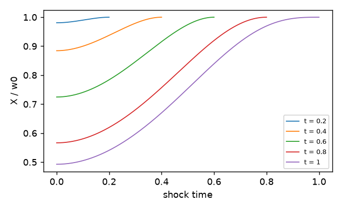
Each curve fixes one date t; the horizontal axis is the shock time s, the moment a shock
struck. The distance t - s is that shock's age.
Along one curve, the observation date stays fixed while the shock's age varies:
k = res.kernel("X", "w0")
k.at(1.0, 1.0)      # +1.0000   at t=1, a shock just struck: it moves X one for one, at once
k.at(1.0, 0.5)      # +0.7539   at t=1, about three-quarters of a shock of age 0.5 remains
k.at(1.0, 0.0)      # +0.4926   at t=1, a shock of age 1.0 is still half there
To follow a single shock over time, fix s and vary t:
k.at(0.50, 0.5)     # +1.0000   the shock at s=0.5, the instant it lands
k.at(0.75, 0.5)     # +0.8773   the same shock, a quarter later
k.at(1.00, 0.5)     # +0.7539   the same shock at the end of the game
A positive value means the state is still displaced in the direction of the shock. The decay in
either reading reflects the players' control actions: without them, X would retain the full
effect of the shock, since the state has no other restoring force.
The control response has the opposite sign:
d = res.kernel("D1", "w0")
d.at(0.5, 0.5)      # +0.0000   age 0:  no reaction at all to a shock just struck
d.at(0.5, 0.4)      # -0.2256   age 0.1: player 1 pushes back, against the shock
d.at(1.0, 0.9)      # +0.0000   at t = T there is no horizon left to control
The reaction at age zero is zero because learning about X requires accumulating observations.
The subsequent negative response counteracts the positive shock.
kernel() returns the closed-loop response to primitive shocks. The implementable strategy is
res.maps["player1"]: the weights the player puts on its own signal history. Kernels describe
the effects of shocks; maps describe how the player uses its observations.
Change one thing
Give player 1 four times the precision, keeping the other model parameters fixed, and solve again:
sharper = ns.solve(model.with_params(p1=12.0))
sharper.require_ok()
sharper.costs      # player1 0.359950,  player2 0.331103
| agent | cost at p1 = 3 |
cost at p1 = 12 |
change |
|---|---|---|---|
| player1 | 0.396906 | 0.359950 | -9.3% |
| player2 | 0.396906 | 0.331103 | -16.6% |
Both players benefit from player 1's better information. Player 2's cost falls by almost twice as
much: it benefits from a more stable state while player 1 pays for its own control effort.
Both losses place the same weight on deviations of X from zero.
with_params() returns a new model; model is untouched, so you can sweep without rebuilding.
To keep an editable copy of the changed model and load it in a later session:
model.with_params(p1=12.0).save("sharper.yaml")
saved_model = ns.load("sharper.yaml")
Did the required checks pass
res.require_ok() checks more than convergence. A converged solve is a numerical solution, within the
solver's tolerance, of the discretised, truncated model -- which is not the same as the model you
wrote:
- converged -- the fixed-point iteration reached its tolerance.
res.converged. - accepted -- every check a stated policy requires actually passed.
res.diagnostics.assess().
A result can converge on a grid that is too coarse or a lag window that is too short.
Use require_ok() to check the result before using it in a script:
res.require_converged()          # ConvergenceError unless the iteration converged -- convergence only
res.require_ok()                 # the full assessment: raises unless every required check PASSED
When it raises, the message names the check, what it measured and what to change:
res = ns.solve(ns.example("ch3_two_player"))
res.converged                    # True
res.require_ok()                 # DiagnosticsError: converged, but window [failed] WINDOW TOO SHORT
                                 #   (a kernel still moves by 2.4% of its peak over the last tenth
                                 #    of the window: raise horizon.window)
Acceptance means the required numerical checks passed for this solve. It does not establish that the model represents the intended problem. See docs/guards.md for check statuses, policies, and advice on failures.
Which example should I start from
Seven models ship with the package; ns.examples() lists them. After this walkthrough, try
ch1_delayed_finite: it keeps the tracking objective while adding a delay to both controls and
to player 2's observation. Inspect model.describe() and compare its kernels with this game's.
For a different economic application, try ch4_kyle_back next.
Those three are introductory examples with accepted defaults. The remaining four are benchmarks or advanced examples for studying numerical checks and transitions; each documents its flags in its own file. Use the table to choose a model and interpret its default outcome:
| example | the question it asks | horizon | out of the box |
|---|---|---|---|
ch1_two_player_finite |
two players track one state over a fixed period | finite, T = 1 | accepted |
ch1_delayed_finite |
tracking with delayed controls and a delayed observation | finite, T = 1 | accepted; recommended next example |
ch3_two_player |
the same tracking game with no end date | stationary | window too short -- the dissertation's own window; with_stationary(9.0) clears it |
ch4_kyle_back |
an informed trader against a market maker who prices order flow | stationary, discounted | accepted |
kyle_back_prior |
the same, started from a prior on the fundamental | transition | not a minimum -- attributed to a discretisation artifact; see the example's notes |
ch5_cycle_market |
a ring of firms buying and selling with a delivery lag | stationary | under-resolved -- increasing resolution can be expensive; see the example's notes |
ch3_precision_change |
a regime change: one player's precision jumps | transition | several -- see the transition walkthrough for interpretation |
ns.example(name) gives the path and ns.load(...) the model, as above.
Find the names in another model
The strings passed to kernel() and used as keys in costs come from the model. After loading a
file, inspect them before solving; for the first tracking game:
model.state_names                   # ['X']
model.control_names                 # ['D1', 'D2']
model.channels                      # ['w0', 'w1', 'w2']
[agent.name for agent in model.agents]  # ['player1', 'player2']
Use a state or control name as the first argument to res.kernel(), a channel as its optional
second argument, and an agent name in res.costs or res.maps. print(model.describe()) explains
which controls and signal rows belong to each agent. These names belong to the loaded model;
another example may use different ones.
Three objects
The API centres on three objects: a Model describes the game, Numerics specifies how it
is solved, and a Result holds the solution and diagnostics. For example,
ns.solve(model, ns.Numerics(nodes=32)) changes the resolution without changing the game.
The remaining sections provide the reference for these objects.
What a Result holds
res.costs["player1"]         # the cost of each agent (res.cost_kind says what it is)
res.cost_parts["player1"]    # its {"variance", "mean"} parts
res.kernel("X")              # closed-loop kernel of a state, one column per channel; .axes, .at(), .plot()
res.strategy_kernel("D1")    # closed-loop kernel of a control
res.maps["player1"]          # raw strategy g[u][r](b) on the agent's own signal rows
res.foc["player1"]["D1"]     # {"foc", "physical", "wedge"}: the first-order condition decomposed
res.means["X"]               # the mean of a state or control: a constant here, a path on a finite horizon
res.axes                     # the coordinates of kernel(): {"age"} stationary, {"time","age","shock_time"}
                             # on the finite triangle, {"time","shock_time"} for the cell engine
res.times, res.paths         # the paths of a finite horizon
res.numerics                 # the resolved Numerics
res.evaluations, res.seconds, res.residual, res.message
res.world                    # every closed-loop kernel stacked
res.extra                    # the engine's extras
res.diagnostics              # the checks: .statuses, .rows, .flags, .assess(policy), .summary()
res.summary(); res.to_dict() # the text report; the JSON-ready payload
res.refine() re-solves at 1.5 times the nodes and returns a Refinement (.cost_change,
.kernel_change, .resolved, .fine -- the finer Result itself). res.stability() returns a
Stability (.radius, .eigenvalues, .verified, .full_response, .adjusted_response).
The model file
name: ch4_kyle_back
params: {eps: 0.2, rho: 0.5, gamma1: 1.0, sigma_V: 1.0, sigma_Z: 1.0}
channels: [wV, wZ, w1]                          # Brownian channels
states:
  V: {drift: {}, noise: {wV: sigma_V}}          # dV = sigma_V dW_V (random walk on the window)
agents:
  market_maker:
    controls: [P]
    myopic: true                                # competitive: no continuation effects of own action
    signals:
      flow: {drift: {D1: 1.0}, noise: {wZ: sigma_Z}}
    loss: [[1.0, P, P], [-2.0, P, V]]           # (P - V)^2  ->  P = E[V | flow history]
  trader1:
    controls: [D1]
    signals:
      y1: {drift: {V: gamma1, P: "-gamma1"}, noise: {w1: 1.0}}
      flow: {drift: {}, noise: {wZ: sigma_Z}}   # sees the flow net of its own orders
    loss: [[-1.0, D1, V], [1.0, D1, P], [eps, D1, D1]]
horizon: {kind: stationary, discount: rho, window: 8.0}
numerics: {nodes: 24}
An atom names a state, control, or definition; name@tau refers to its value tau earlier.
A state's drift is linear in these atoms, with an optional const term. Its noise specifies
the loading on each Brownian channel. Finite-horizon states can also have an initial value.
Signal rows have a drift, a noise loading, and an optional observation delay.
Losses sum quadratic terms [coef, a, b] and linear terms [coef, a]. Linear loss terms,
constant drifts, and initial states affect only the means. Coefficients can be expressions in
the model's parameters. ties imposes a shared strategy on a group of agents, and numerics
sets the solver options.
See docs/model_file.md for each field's type and default.
noisestate schema model prints the JSON Schema.
The horizon: two different lengths
horizon specifies the time structure of the game. Its two length parameters have different roles:
windowis L, the lag-truncation length: how far back a strategy may look. Stationary models have one; transitions have one too.Tis the terminal time: the end of the interval that is solved for. Finite horizons and transitions have one. On a finite horizon the game does end atT. On a transition it usually does not:Tis where the solved path stops and a stationary continuation takes over on a buffer after it.
horizon: {kind: stationary, discount: 0.5, window: 8.0}    # L = 8, no terminal time
horizon: {kind: finite, T: 1.0}                            # ends at 1, no lag window
horizon: {kind: transition, T: 6.0, window: 3.0, past: ...}   # both
discount is the rate rho and defaults to 0. For stationary models, this gives the formal
average-cost equations. The stationary verification assumes rho > 0; at zero discount, the
finite lag window substitutes numerically for the transversality condition. A converged result
can therefore depend on the window rather than represent the untruncated game.
Stationary res.costs reports flow loss per unit time, even at a positive discount. The rate
affects the equilibrium through the first-order conditions, but the reported cost is not the
discounted objective. Finite-horizon costs are discounted integrals over [0, T]. Check
res.cost_kind when comparing results. Further details are in
docs/limits.md.
The three horizon kinds have separate Python types. with_stationary(L), with_finite(T), and
with_transition(T, past) update a horizon of the corresponding kind. Use with_horizon(obj)
to replace it with a different kind. Requesting a length that does not apply raises an error.
model.with_stationary(9.0)                       # a stationary model's lag window
model.with_finite(6.0)                           # a finite model's terminal time
model.with_horizon(ns.Finite(T=6.0))             # replace the horizon, whatever it was
Other ways to build a model
Models can also be written as Python expressions or assembled with a builder. Both produce a
Model whose to_dict() method returns the same structure used by the YAML format.
As equations
Use Param, State, Control, Signal, Agent, and shocks to write the model as expressions.
In an assignment to a state's drift, quantity terms define the drift, shock terms define the
noise loading, and a constant becomes const. A signal is a linear expression containing at
least one shock; a loss is quadratic in the quantities.
Constant loss terms are omitted: (X - 1)**2 becomes X^2 - 2X, with the omission recorded in
model.notes. Write x.lag(tau) for the YAML atom x@tau.
import noisestate as ns
from noisestate import Param, State, Control, Signal, Agent, shocks
r1, r2, p1, p2, sigma = Param.many(r1=0.1, r2=0.1, p1=3.0, p2=3.0, sigma=1.0)
w = shocks("w0", "w1", "w2")
X = State("X"); D1, D2 = Control("D1"), Control("D2")
X.drift = D1 + D2 + sigma * w.w0
player1 = Agent("player1", controls=[D1], signals=[Signal("y1", p1**0.5 * X + w.w1)], loss=X**2 + r1 * D1**2)
player2 = Agent("player2", controls=[D2], signals=[Signal("y2", p2**0.5 * X + w.w2, delay=0.5)], loss=(X - 1)**2 + r2 * D2**2)
game = ns.Model("ch1", states=[X], agents=[player1, player2], horizon=ns.Stationary(window=3.0))
print(game.describe())
eq = game.solve(ns.Numerics(nodes=16, unit=0.5))
eq.require_ok(); eq.costs["player1"]; eq.cost_parts["player1"]; eq.means["X"]
k = eq.kernel("X", "w0"); k.values; k.axes; k.at(0.7)
for point in game.sweep(p1=[0.3, 1, 3, 10]): point.value, point.result, point.jump
game.save("ch1.yaml"); ns.Model.load("ch1.yaml")
with ns.using_settings(second_order_tol=1e-3): game.solve()
The model collects the shocks and parameters used in its expressions. Channels retain their
shocks() order, and Param.many returns parameters in argument order. Coefficients support
+ - * / ** and sqrt exp log sin cos tanh abs min max; saved expressions preserve their parameter
dependence, so p1**0.5 is written as "sqrt(p1)".
Use define(name, expr) for a named definition, ns.Finite(T) or
ns.Transition(T, past=..., continuation=...) for other horizons, and numerics= for solver
options. examples/expr_examples.py expresses all shipped examples this way;
tests/test_expr.py checks them against their YAML equivalents. Models are saved as YAML.
With ModelBuilder
import noisestate as ns

b = ns.ModelBuilder("one_agent", a=1.0, r=0.5)
b.channel("w", "v")
b.state("X", drift={"X": "-a", "D": 1.0}, noise={"w": 1.0})
b.agent("me", controls=["D"], loss=[[1.0, "X", "X"], ["r", "D", "D"]])
b.signal("me", "y", drift={"X": 1.0}, noise={"v": 1.0})
b.stationary(discount=0.1, window=8.0, nodes=16)
res = ns.solve(b)
examples/make_ch5_cycle_market.py builds an N-firm cycle in a loop; b.finite(T, nodes) and
b.transition(T, nodes, past=..., continuation=...) set the other horizons and b.numerics(**fields)
the rest of the block.
Changing what agents see
with_signal() adds an observation row and any new noise channels, returning a new model.
By default, every agent observes the row. with_signals() adds several rows at once;
without_signal() removes a row.
public = game.with_signal("flow", drift={"D1": 1, "D2": 1}, noise={"w_flow": 1})
player1_only = game.with_signal("flow", drift={"D1": 1}, noise={"w_flow": 1}, audience="player1")
same_row = game.with_signal(Signal("flow", D1 + D2 + w.w_flow))      # the expression form's own type

study = ns.compare({"none": game, "balanced": public, "only player 1": player1_only},
                   baseline="none", stability=True)
print(study.summary())
study["balanced"].result                 # the ordinary noisestate Result
study["balanced"].cost_changes           # each agent against the baseline
study["balanced"].dynamics               # full and 50%-adjusted best responses
study.to_dict(include_results=False)     # compact, JSON-ready comparison
audience= is "all", one agent name or an iterable of names. compare() solves structurally
different scenarios independently and requires the same agents, horizon, discount and window so its cost
changes compare like with like. Adjustment convergence is certified only when the computed leading
spectrum bounds the omitted modes; otherwise adjusted_response says not certified.
Transitions
A transition describes the path after a regime change at time zero. The solver computes this path on [0, T], inheriting the effects of earlier shocks from a past. Supply the old model, its converged result, or initial shocks representing a prior on the state.
With continuation: stationary, the new model's stationary equilibrium supplies the continuation
on a buffer [T, T + L]. With continuation: end, the game ends at T.
import noisestate as ns

res = ns.solve(ns.example("ch3_precision_change"))             # the file form: horizon.past, horizon.continuation
old = ns.solve(ns.example("ch3_two_player"))
new = ns.load(ns.example("ch3_two_player")).with_params(p1=10.0)
res = ns.transition(old, new, T=6.0, numerics={"nodes": 12})   # solves the new stationary equilibrium and the transition
res = ns.transition(old, new, settle=1e-4, numerics={"nodes": 12})   # or finds T: a march (res.extra["window"], res.march)
res.settled, res.excess_costs, res.loss_path["player1"], res.belief_error("player2", "X")
Every transition starts from the continuation's stationary maps. Two exact identities check the construction: a model as its own past and continuation returns its stationary kernels on every node, and a prior on the state of the one-agent model reproduces the Kalman filter. The construction, the result's fields and the two shipped examples are in docs/transitions.md.
Sweeps and interactive use
import noisestate as ns

rows = ns.sweep(ns.example("ch4_kyle_back"), "eps", [0.2, 0.1, 0.05])   # each point warm-started
rows[-1].result.summary(); rows[-1].change, rows[-1].jump, rows[-1].value
Each point is a SweepPoint (.param, .value, .result, .change, .jump, .converged,
.evaluations, .seconds) and starts from a secant extrapolation of the previous two equilibria,
which carries the Kyle-Back sweep down to a trading cost of 0.01 where a plain restart fails. A row
whose change is more than five times the sweep's median is a jump, so a branch change between
neighbouring points is visible instead of plotted as a curve.
For interactive use, a solve can have evaluation and time limits and report its progress:
log = []
res = ns.solve(ns.example("ch3_two_player"), max_evaluations=3, deadline=30.0,
               progress=lambda ev: log.append(ev["residual"]), diagnostics=False)
res.converged, res.message          # False, the bound that stopped it; nothing raises
max_evaluations limits best-response evaluations; deadline limits elapsed time in seconds.
If either limit stops the solve, it returns the best iterate with converged=False and identifies
the limit in res.message.
progress is called after every evaluation with {"evaluation", "residual", "phase", "seconds"}; an
exception it raises cancels the solve. diagnostics=False skips the checks at the end (res.foc and
res.second_order stay empty, those checks report skipped) and halves a warm-started re-solve.
start_policy="coarse" solves first at half the nodes; start_from= takes explicit kernels or maps.
sweep(..., solve_kw={...}) forwards these to every point. Grids and their operator caches are shared
across solves in a process (ns.clear_grid_cache() releases them).
The guards
res.diagnostics.rows lists every check as a row {name, value, threshold, ok, flag, advice} plus the
stable code, category, severity, meaning, action and suggested_options fields the payload
carries; summary() prints the ones that fail. The full descriptions, with thresholds and advice, are
in docs/guards.md.
Resolution. The representation error of the action kernels on the seen rows above 1e-6 prints
UNDER-RESOLVED (representation error 1.3e-05: raise numerics.nodes). solve(..., refine=True) or
res.refine() re-solves at 1.5 times the nodes and reports the change of every cost and kernel, with
resolved=False when either moves more than its tolerance.
Window. On the stationary engine a kernel still moving by more than 2% of its peak over the last
tenth of the window prints WINDOW TOO SHORT (a kernel still moves by 4.1% of its peak over the last tenth of the window: raise horizon.window): the equilibrium solved is that of the model truncated at
horizon.window. The Kyle-Back example with rho: 0 is flagged (its kernels are window artefacts);
it ships with rho: 0.5. For a stationary-window failure the solver compares kernel changes over the
last four tenths of the existing window, reports their median decay ratio and projects the tail at
twice the window, with a benchmark range. A tail whose increments are not shrinking suppresses the
automatic extension suggestion and instead warns that the stationary problem may not exist, as in
undiscounted Kyle-Back.
Second order. Negative curvature can indicate a saddle or a discretisation artifact.
res.refine() re-solves on a finer grid and records the curvature there
(res.refinement.curvature). Curvature that shrinks towards zero under refinement indicates a
discretisation artifact. In examples/kyle_back_prior.yaml, the corresponding direction sits on
the triangle's diagonal a = t and alternates in sign between neighbouring age nodes. The smallest
curvature runs -1.45e-02, -1.02e-02, -8.26e-03, -6.71e-03, -5.63e-03 at 8, 12, 16, 20 and 24 nodes,
about n^-0.85. The objective is a quadratic form in the agent's strategy, and a smallest curvature
below -1e-4 of the largest prints
NOT A MINIMUM (the best response of 'trader1' is a saddle: its loss is not convex in its own strategy, smallest curvature -1.8e-03 of the largest). A negative direction that is positive on a
window longer by two lags is reported as window edge: ... a truncation of the lagged loss terms at the edge, not a saddle instead. The check also applies with a positive discount: the discounted objective is
a quadratic form whose joint running Hessian carries no discount, since rho enters only as the
strictly positive weight e^{-rho t}, so the verdict is the same at every rho and the check is
made on the average-cost system. The cell engine is the one that reports unsupported here: it
builds no second-order form at all.
Settled. A transition whose maps on [T - L, T] are more than 1e-4 of their peak from the
stationary continuation prints TRANSITION NOT SETTLED by T - L and suggests a larger --T; the
past's and the continuation's own window tails are echoed as PAST WINDOW TOO SHORT and
CONTINUATION WINDOW TOO SHORT, which suggest --past-window L and --continuation-window L.
Because the buffer reads both stationary regimes over the same ages, the latter enlarges their shared
lag window.
Stability. res.stability() (or solve(..., stability=True)) reports the spectral radius of the
best-response map, best-response dynamics UNSTABLE (spectral radius 1.400) above one: the Kyle-Back
equilibrium converges under Anderson mixing while naive best-response adjustment would not find it.
The classification is withheld unless the point is a verified equilibrium; the spectrum is reported
either way.
What the model rejects. A misspelled key, an unused channel or parameter, a control that does not
enter its owner's loss, a zero noise loading, a lag or delay not below the window, and a singular
best-response system (a control with no quadratic term in its current value, two rows carrying the same
information) are refused with a message naming the item; model.notes and noisestate validate say
what the numbers are (flow losses per unit time or discounted integrals, a random walk pinned at 0).
Settings
The tuning constants live in one frozen dataclass, noisestate.Settings, each with its default and a
one-line meaning: the outer fixed point (anderson_m 15, anderson_iters 150, ...), the best response
(foc_rcond 1e-10, foc_dense_max 500, ...), the second-order check (second_order_tol 1e-4, ...),
the means and the result's checks (resolution_tol 1e-6, window_tail_tol 0.02, settled_tol 1e-4,
...). They are the settings field of Numerics: ns.Numerics(settings=ns.Settings(second_order_tol=1e-3)),
or {"settings": {"second_order_tol": 1e-3}}; the fields that differ from the defaults are recorded in
res.numerics and the payload, so refine(), stability() and a re-solve from the payload keep them.
The table is docs/settings.md.
Errors
Exception types distinguish invalid inputs from solver failures. A ValueError is a model problem: a file that does not
validate, a parameter that is not the model's, a lag off the panels, a singular best-response system, a
solve bound out of range. A TypeError is a wrong argument: an unknown solve option (the message names
the Numerics field it belongs to, or the Numerics(settings=...) route for a Settings field),
naive_observers that is not a mapping. A NotImplementedError is a feature the engine does not have
(leads on the finite engines); a past on the cell engine is a ValueError from the numerics
(numerics.engine 'cells' solves a finite horizon only). A RuntimeError is a solver problem: a Krylov
best response not converging, a non-finite value from the best-response map.
ResultValidationError is the base class for two distinct result-validation exceptions:
ConvergenceError--- the iteration did not converge. Fromrequire_converged(), and fromrequire_ok()when convergence is what blocked.DiagnosticsError--- it converged, but a required check did not pass. Only fromrequire_ok(), and it carries theAssessmentas.assessment.
Catching ConvergenceError therefore does not catch a diagnostic failure; catch ResultValidationError
for both. A fixed point that does not reach tol, or is stopped at max_evaluations or deadline,
does not raise on its own: solve() returns the result with converged=False and res.message, and
sweep() records the row and goes on. converged means the residual (the norm of the update over the
larger of one and the norm of the iterate) is at or below tol.
The command line
noisestate validate examples/ch4_kyle_back.yaml            # the schema, then the model's own checks; prints the notes
noisestate describe examples/ch4_kyle_back.yaml            # the equations, delays, losses and conventions
noisestate solve examples/ch4_kyle_back.yaml -o kb.json --plot kb.pdf --param rho=0.5 --nodes 32
noisestate solve examples/ch3_two_player.yaml --refine --stability --require-ok --diagnostics
noisestate sweep examples/ch4_kyle_back.yaml eps 0.2,0.1,0.05 -o sweep.json
noisestate transition examples/ch3_two_player.yaml new.yaml --T 6 --nodes 12 -o change.json
noisestate transition examples/ch3_two_player.yaml new.yaml --settle 1e-4 --nodes 12   # T found by the march
noisestate schema model > model.schema.json                # JSON Schema (draft 2020-12); also: schema payload
noisestate plot kb.json kb.pdf                             # plots the saved result; --re-solve reproduces the solve first
noisestate plot-sweep sweep.json sweep.png
noisestate --version
solve takes --engine, --tol, --max-evaluations, --deadline and -v as well, and the two
horizon lengths under their own names: --window L (the lag-truncation length, stationary and
transition models) and --T (the terminal time, finite and transition models). Asking for the one a
model's kind does not have is an error that names the other.
The exit status is 0 for a converged solve (a sweep: every point converged), 1 for a solve that ran but
did not converge (the summary is still printed and -o still written), and 2 for a usage error or an
error the package raises, printed as error: ... on stderr. --require-ok makes a diagnostically
unaccepted result exit 1 as well, which is what a batch script wants; --policy exploratory asks for
the weaker standard by name. A check the engine cannot compute is reported as cannot be checked here
rather than as a failure, and says whether any setting could change it. The JSON written by -o is
res.to_dict(), documented key by key in docs/payload.md; it validates against
noisestate.schema("payload").
Working on noisestate
python -m venv .venv && .venv/bin/pip install -e ".[dev]"
./run-tests                        # the fast suite, about 2 minutes
NOISESTATE_SLOW=1 ./run-tests      # everything, about 6 minutes
Run the suite through ./run-tests, not pytest directly. The wrapper prevents overlapping test
runs and limits BLAS threads to keep timings comparable and avoid thread overhead on small solves.
Where things are
- docs/model_file.md: every key of a model file, with its type and default.
- docs/payload.md: every key of
to_dict()and the CLI's JSON. - docs/transitions.md: the transition engine in full, with the two examples.
- docs/guards.md: the checks, their statuses, thresholds and advice.
- docs/settings.md: the tuning constants.
- docs/api.md: every public function and method, with its use case.
- docs/validation.md: what the tests reproduce, with the numbers.
- docs/method.md: how it works, the means, the grids, the stability guarantees.
- docs/limits.md: what the grammar and the engines do not do.
- docs/architecture.md: the modules, one best response and one transition through them.
- docs/design/: the design record, and the dated reviews behind it.
- CHANGELOG.md: public releases, starting with 1.0.0.
1 maintainer

Release files for noisestate 1.0.1
For a detailed explanation of source distributions (sdists) and built distributions (wheels), please see the package formats documentation.
Source distribution (sdist)
| File | Size | Uploaded | |
|---|---|---|---|
| noisestate-1.0.1.tar.gz | 291.1 kB | Details |
Built distribution (wheel)
| File | Interpreter | ABI | Platform | Reset |
|---|---|---|---|---|
| noisestate-1.0.1-py3-none-any.whl | Python 3 | none | any | Details |
Total release size: 579.4 kB
Release files / noisestate-1.0.1.tar.gz
| Download URL | noisestate-1.0.1.tar.gz |
|---|---|
| Size | 291.1 kB |
| Tags | Source |
|
SHA-256 checksum How to use checksums |
dab88b3786432ec44955cf302c66257745c02996f0ab34d68d75dcd1c896f051
|
|
BLAKE2b-256 checksum How to use checksums |
74033454740ee554c790569799e921f7fedd7f4cbd909b6bee47882b18e4b0af
|
| Upload date | |
|
Uploaded using Trusted Publishing? What is trusted publishing? |
Yes |
| Uploaded via |
twine/7.0.0 CPython/3.13.14
|
Provenance
Provenance describes where a file came from. On PyPI, provenance is shared via attestations, which provide a verifiable record of the build or publishing details. View details, limitations and caveats.


PyPI Publish Attestation
PyPI verified that this artifact, at this checksum, originated from the publisher listed below.
Signed by GitHub Actions, verified by PyPI on Sep 23, 2026.
Transparency logRelease files / noisestate-1.0.1-py3-none-any.whl
| Download URL | noisestate-1.0.1-py3-none-any.whl |
|---|---|
| Size | 288.4 kB |
| Tags | Python 3 |
|
SHA-256 checksum How to use checksums |
cc0ade934a7bbbacb0c608134525e18d969a048bb1947c8c841b461c40f5f589
|
|
BLAKE2b-256 checksum How to use checksums |
132e9d0f167298d1ae2ca092d13142a174c8f625fb79140fda79a77d7749641d
|
| Upload date | |
|
Uploaded using Trusted Publishing? What is trusted publishing? |
Yes |
| Uploaded via |
twine/7.0.0 CPython/3.13.14
|
Provenance
Provenance describes where a file came from. On PyPI, provenance is shared via attestations, which provide a verifiable record of the build or publishing details. View details, limitations and caveats.
PyPI Publish Attestation
PyPI verified that this artifact, at this checksum, originated from the publisher listed below.
Signed by GitHub Actions, verified by PyPI on Sep 23, 2026.
Transparency log













