
NoMaSS: Non-Markovian Stochastic Simulation



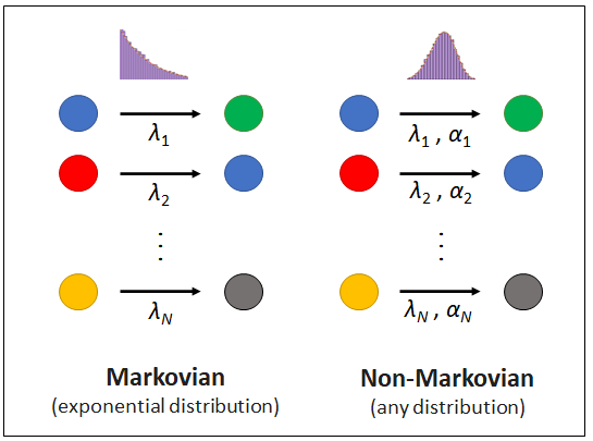
Discrete stochastic processes are widespread in nature and in human-made systems, with applications in physics, biochemistry, epidemiology, social dynamics and finance. In most of these systems the dynamics cannot be described with memoryless (Markovian) interactions, and simulating them requires dedicated numerical tools.
NoMaSS is a practical and scalable Gillespie-based framework to simulate non-Markovian reaction networks with arbitrary inter-event time distributions. It implements three exact methods that can be mixed freely in the same model, one per reaction channel:
- MOSAIC (rejection based, [1, 2]): propose events at an upper bound of the rate and accept them with the ratio of the true hazard to the bound.
- Laplace Gillespie [3]: give every reactant a Poisson rate drawn from the mixing density of its waiting-time distribution.
- DelaySSA [4]: draw the waiting time when a reactant enters a channel and schedule the event in a priority queue.
The methods, their accuracy and their speed are described in the accompanying paper [1].
Installation
NoMaSS is deliberately lightweight: the efficiency of the framework lies in the algorithms rather than in compiled extensions, so the engine is pure Python and relies only on the standard scientific stack. Python 3.9 or later is required.
pip install nomass
To work on the code or run the scripts of the paper, clone the repository and install it in editable mode:
git clone https://github.com/AI-SysBio/NoMaSS.git
cd NoMaSS
pip install -e .[test,paper]
Check that everything works with
python examples/toy_example.py
Quick start
The example below (examples/toy_example.py) simulates a small network where each channel uses a different method:
import nomass

# Reaction channels: one waiting-time distribution and one method each
r1 = nomass.Reaction_channel('A -> B', rate=1, shape_param=20, distribution='Gamma', method='Delay')
r2 = nomass.Reaction_channel('B -> C + A', rate=4, shape_param=5, distribution='Weibull', method='MOSAIC')
r3 = nomass.Reaction_channel('C -> 0', rate=0.03, shape_param=0.5, distribution='Gamma', method='Laplace')
r4 = nomass.Reaction_channel('A + B -> 0', rate=0.03)   # two reactants: Poisson process

# Initial population (every species must be listed)
N_init = {'A': 300, 'B': 0, 'C': 0}

# Build and run the model
sim = nomass.Gillespie_simulation(N_init, [r1, r2, r3, r4],
                                  Tend=10,            # length of the simulation
                                  N_simulations=20,   # number of independent realisations
                                  timepoints=100,     # number of recorded time points
                                  unit='h')           # time unit (plots only)
populations = sim.run_simulations()   # array (N_simulations, timepoints, species + total)

# Plot the results
sim.plot_inter_event_time_distribution()
sim.plot_populations()
The simulation runs in a few seconds and produces the figures below (pass verbose=False to silence the progress output).
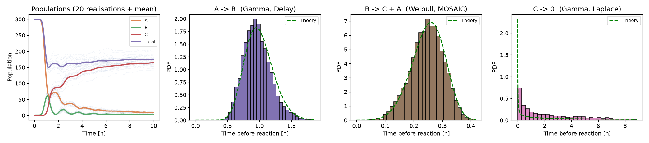
The oscillations created by the nearly deterministic Gamma waiting times are clearly visible. The theoretical distributions do not match the simulated ones exactly, even with many realisations, and this is expected: species A and B are reactants of two channels at the same time, and the theoretical curve is the distribution the channel would have if it were the only process acting on its reactant. The accuracy of each method is demonstrated in [1] and [2].
Reactions are written as strings: 'A + B -> C', '0 -> A' (creation), 'A -> 0' (degradation), '2 A -> B' (stoichiometry). The plotting methods return their matplotlib figure and axes, so pass show=False to customise a figure before displaying it.
Choosing a method
| Method | Set with | Best for | Limitations |
|---|---|---|---|
| MOSAIC (rejection) | method='MOSAIC' |
Large populations, state-dependent rates, any distribution with a bounded hazard | Hazard must be finite at t = 0 (Gamma and Weibull need a shape ≥ 1) |
| Laplace Gillespie | method='Laplace' |
Heavy-tailed or decreasing hazards (Gamma/Weibull with shape < 1, Lomax), state-dependent rates | Only distributions whose survival function is a mixture of exponentials |
| DelaySSA | method='Delay' |
Any distribution when rates are constant | Waiting times are frozen when drawn, so rates that change over time are not followed |
When method is omitted, NoMaSS uses MOSAIC if the hazard is bounded and Laplace Gillespie otherwise. Channels with zero or several reactants are always Poisson processes with propensity rate × product of the reactant counts, because the waiting time of an individual is not defined in that case.
A Gamma waiting time with an integer shape can also be embedded in a chain of exponential stages (hidden Markov embedding); examples/erlang_embedding.py compares the two descriptions.
Supported distributions
| Distribution | MOSAIC | Laplace | DelaySSA |
|---|---|---|---|
| Exponential | ✅ | ✅ | ✅ |
| Gamma | ✅ (α ≥ 1) | ✅ (α ≤ 1) | ✅ |
| Weibull | ✅ (α ≥ 1) | ✅ (α ≤ 1) | ✅ |
| Gaussian / Normal | ✅ | ❌ | ✅ |
| Lognormal | ✅ | ❌ | ✅ |
| Cauchy | ✅ | ❌ | ✅ |
| Power law, Pareto type I | ✅ | ❌ | ✅ |
| Power law, Lomax (Pareto type II) | ✅ | ✅ | ✅ |
Every distribution is parameterised by a nominal rate λ, the inverse of the mean waiting time (or of the median when the mean is undefined), and a dimensionless shape_param α (full details in Table S1 of [1]):
| Distribution | rate |
shape_param |
|---|---|---|
| Exponential | 1 / mean | unused |
| Gamma | 1 / mean | shape α |
| Weibull | 1 / mean | shape k |
| Gaussian | 1 / mean | std / mean |
| Lognormal | 1 / mean | std / mean |
| Cauchy | 1 / median | scale / median |
| Pareto type I | 1 / median | tail index α |
| Lomax | 1 / median | tail index α |
Gaussian and Cauchy waiting times are truncated to non-negative values. Aliases such as 'exp', 'norm', 'lognorm' and 'weib' are accepted. Requesting a combination that a method does not support raises an error at channel creation. examples/all_distributions.py runs a cycle through all eight distributions.
State-dependent waiting times
Pass update_function to change the rate or shape_param of any channel after every iteration, for example to implement feedback or resource limitation (examples/state_dependent_rates.py):
def update_rates(sim):
    N = sim.reactant_population['Cell']
    sim.reaction_channel_list[0].rate = r0 * (1 - N / K)   # logistic growth

sim = nomass.Gillespie_simulation({'Cell': 5}, [division], Tend=25, update_function=update_rates)
populations = sim.run_simulations()
MOSAIC and Laplace Gillespie follow such changes exactly (Laplace rates are rescaled when the rate changes and redrawn when the shape changes). Delay-based channels draw their waiting time once, when the reactant enters the channel, so they cannot follow parameters that change afterwards: avoid method='Delay' for rapidly changing systems.
Individual properties
Every individual is a nomass.Reactant object that can carry arbitrary attributes. The on_reaction hook is called after each accepted reaction with the consumed and produced individuals, which is where properties are set or inherited (examples/individual_properties.py):
def inherit(sim, channel, consumed, produced):
    if channel is division:
        for daughter in produced:
            daughter.generation = consumed[0].generation + 1

sim = nomass.Gillespie_simulation({'Cell': 20}, [division, death], Tend=6, on_reaction=inherit)
Set transfer_identity=True on a channel such as 'Gon -> Gon + mRNA' to keep the same individual (with its properties and the clocks of its other channels) instead of replacing it. For kinetic laws that are not proportional to the reactant counts, subclass Gillespie_simulation and override compute_propensities; the full API is described in docs/api.md, and the hazards, samplers and Laplace mixing densities of all distributions are in nomass/distributions.py.
Repository layout
nomass/        the engine (distributions and simulation)
docs/          API reference (docs/api.md)
examples/      short runnable examples
paper/         scripts, data and precomputed results reproducing the paper's figures
tests/         pytest suite (pytest -q)
The biochemical systems of the paper (bacterial growth, stem cell differentiation and RNA transcription) live in paper/, with a figure-to-script table in paper/README.md and the article with its supplementary material in paper/Pelissier2026_NoMaSS_main_and_SI.pdf.
Citation
If you use NoMaSS, please cite (full text with supplementary material: paper/Pelissier2026_NoMaSS_main_and_SI.pdf)
Pélissier A., Phan M., Beerenwinkel N., Rodríguez Martínez M. Gillespie-based simulation and inference for non-Markovian stochastic reaction networks. Briefings in Bioinformatics 27(5), bbag486 (2026). doi:10.1093/bib/bbag486
@article{pelissier2026nomass,
  title   = {Gillespie-based simulation and inference for non-Markovian stochastic reaction networks},
  author  = {P{\'e}lissier, Aur{\'e}lien and Phan, Miroslav and Beerenwinkel, Niko and Rodr{\'i}guez Mart{\'i}nez, Mar{\'i}a},
  journal = {Briefings in Bioinformatics},
  volume  = {27},
  number  = {5},
  pages   = {bbag486},
  year    = {2026},
  doi     = {10.1093/bib/bbag486}
}
Questions are welcome, feel free to open an issue or drop me an email.
References
[1] Pélissier A., Phan M., Beerenwinkel N., Rodríguez Martínez M. Gillespie-based simulation and inference for non-Markovian stochastic reaction networks. Briefings in Bioinformatics 27(5), bbag486 (2026). doi:10.1093/bib/bbag486
[2] Pélissier A., Phan M., Le Bail D., Beerenwinkel N., Rodríguez Martínez M. Unifying non-Markovian dynamics and agent heterogeneity in scalable stochastic networks. Nature Communications 17, 3345 (2026). doi:10.1038/s41467-026-69817-y
[3] Masuda N., Rocha L. E. C. A Gillespie algorithm for non-Markovian stochastic processes. SIAM Review 60(1), 95-115 (2018). doi:10.1137/16M1055876
[4] Anderson D. F. A modified next reaction method for simulating chemical systems with time dependent propensities and delays. The Journal of Chemical Physics 127(21), 214107 (2007). doi:10.1063/1.2799998
1 maintainer

Metadata
1 maintainer
Release files for nomass 1.0.0
For a detailed explanation of source distributions (sdists) and built distributions (wheels), please see the package formats documentation.
Source distribution (sdist)
| File | Size | Uploaded | Provenance | Actions |
|---|---|---|---|---|
| nomass-1.0.0.tar.gz | 31.0 kB | Without provenance | Details for nomass-1.0.0.tar.gz |
Built distribution (wheel)
| File | Interpreter | ABI | Platform | Actions Reset |
|---|---|---|---|---|
| nomass-1.0.0-py3-none-any.whl | Python 3 | none | any | Details for nomass-1.0.0-py3-none-any.whl |
Total release size: 54.5 kB
Release files / nomass-1.0.0.tar.gz
| Download URL | nomass-1.0.0.tar.gz |
|---|---|
| Size | 31.0 kB |
| Tags | Source |
|
SHA-256 checksum How to use checksums |
4c5f4d631fbfdf7922e30abedc28663a42a882c274990e6c017c14cebedb7618
|
|
BLAKE2b-256 checksum How to use checksums |
6536d457d141edb4368e27b095ebe4418226ec9c4188ff9bb230d659712f53c9
|
| Upload date | |
|
Uploaded using Trusted Publishing? What is trusted publishing? |
No |
| Uploaded via |
twine/7.0.0 CPython/3.12.14
|
Release files / nomass-1.0.0-py3-none-any.whl
| Download URL | nomass-1.0.0-py3-none-any.whl |
|---|---|
| Size | 23.5 kB |
| Tags | Python 3 |
|
SHA-256 checksum How to use checksums |
f522f16cab3bcd346ea4c104be89d651ec868d98ff24f9056a2219688230db34
|
|
BLAKE2b-256 checksum How to use checksums |
ce864192e7e2cf61d2c40b724ca5b664df153054a34756886196dc3ecbb84173
|
| Upload date | |
|
Uploaded using Trusted Publishing? What is trusted publishing? |
No |
| Uploaded via |
twine/7.0.0 CPython/3.12.14
|
Security for nomass 1.0.0
Provenance
Provenance describes where a file came from. On PyPI, provenance is shared via attestations, which provide a verifiable record of the build or publishing details. View details, limitations and caveats.
No provenance found
None of the files in this release were uploaded with provenance metadata.
A note on package security
PyPI is a repository for distributing packages, not a service for auditing them. While third-party security researchers and our staff do their best to detect and remove malicious packages, PyPI cannot guarantee the quality, security or suitability of any given package.
To learn more about protecting yourself from malicious actors, visit our package security documentation.













