
NsgOrcFx
Library of tools for the OrcaFlex API
This package wraps the original API from Orcina (OrcFxAPI) to include:
- methods: pre- and post-processing tools such as line selection, load case generation, modal and fatigue analysis
- coding facilities: auto-complete and hints with descriptions in IDE
All the attributes and methods from the source (OrcFxAPI) still accessible in the same way.
Installation:
pip install --upgrade NsgOrcFx
Example 1 - Auto-complete feature of IDE (e.g. VS Code and Spyder)
import NsgOrcFx

model = NsgOrcFx.Model()
line = model.CreateLine()
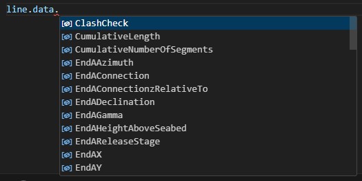
The data name may be found in the data attribute with the auto complete of the IDE (e.g., Visual Studio Code, Spyder, and PyCharm).
In addition, a hint shows the description of the parameter (mouse cursor stopped in the data name).
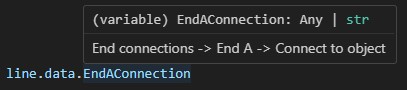
In the exemple below, data names of general, environment, and line objects are accessed
model.general.data.ImplicitConstantTimeStep = 0.01 # data from general object
model.environment.data.WaveHeight = 5.0 # data from environment object
line.data.EndAConnection = 'Anchored' # data form the line object
The line could be alse located by name with the following method. Although it could be done with the original method (line = model['Line1']), the new method is recommended to allow the functionality of auto-complete (data attribute)
line = model.findLineByName('Line1')
A list of all lines in the model may be retrieved and then select the first one by
lines = model.getAllLines()
line1 = lines[0]
Example 2 - Reduced simulation time for irregular wave
import NsgOrcFx as ofx

model = ofx.Model()

# set irregular wave
model.environment.data.WaveType = 'JONSWAP'
model.environment.data.WaveHs = 2.5
model.environment.data.WaveGamma = 2
model.environment.data.WaveTp = 8

# set reduced simulation duration with 200 seconds
model.SetReducedSimulationDuration(200)

# save data file to check the wave history
model.Save('reduced.dat')

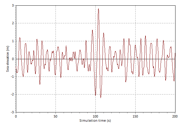
# after executing this code, open the generated data file
# then open Environment -> Waves preview, and set duration of 200s
# click in View profile and observe that the largest event (rise or fall)
# is in the midle of the sea elevation history
Example 3 - Generate load cases
import NsgOrcFx

model = NsgOrcFx.Model()
model.CreateLine()

# list of wave direction, height, and periods to define the Load Cases (LCs)
directions = [0, 45, 90]
heights = [1.5, 2.0, 3.0]
periods = [5, 7, 9]

# Folder to save the generated files (LCs)
outFolder = 'tmp'

# Regular waves
model.GenerateLoadCases('Dean stream', directions, heights, periods, outFolder)
In case of irregular wave:
model.GenerateLoadCases('JONSWAP', directions, heights, periods, outFolder)
To run irregular waves with reduced simulation time, based on the occurance of the largest rise or fall in the specified storm period.
model.GenerateLoadCases('JONSWAP', directions, heights, periods, outFolder, reducedIrregDuration=200)
Example 4 - Calculating modal analysis and getting the normalized modal shape
import NsgOrcFx

model = NsgOrcFx.Model()
model.CreateLine()

modes = model.CalculateModal()

# mode shape index (0 for the 1st)
modeIndex = 0

# mode frequency
freq = modes.getModeFrequency(modeIndex)

# if normalize = True, the displacements will be normalized, so the maximum total displacements is equal to the line diameter
[arcLengths, Ux, Uy, Uz] = modes.GlobalDispShape('Line1', modeIndex, True)
print('Frequency = ', freq, 'Hz')
print(arcLengths, Ux, Uy, Uz)
Example 5 - Defining fatigue analysis and getting the fatigue life calculated
import NsgOrcFx

simFile = r'tests\tmp\fatigue.sim'
ftgFile = r'tests\tmp\fatigue.ftg'

# First, it is necessary a model with simulation complete
model = NsgOrcFx.Model()
model.CreateLine()
model.RunSimulation()
model.Save(simFile)

# The fatigue analysis is defined, including the S-N curve based on the DNV-RP-C203
analysis = NsgOrcFx.FatigueAnalysis()
analysis.data.AnalysisType = 'Rainflow'
analysis.data.LoadCaseCount = 1
analysis.addLoadCase(simFile)
analysis.addSNCurveByNameAndEnv('F3','seawater')
analysis.addAnalysisData()
analysis.Calculate()
analysis.Save(ftgFile)

# Result of fatigue life in each node
lifePerNode = analysis.getLifeList()
print(lifePerNode)
Example 6 - Generates RAO plots from vessel type data
import NsgOrcFx as ofx

model = ofx.Model()

# Create a 'Vessel Type' object with default data
model.CreateObject(ofx.ObjectType.VesselType)

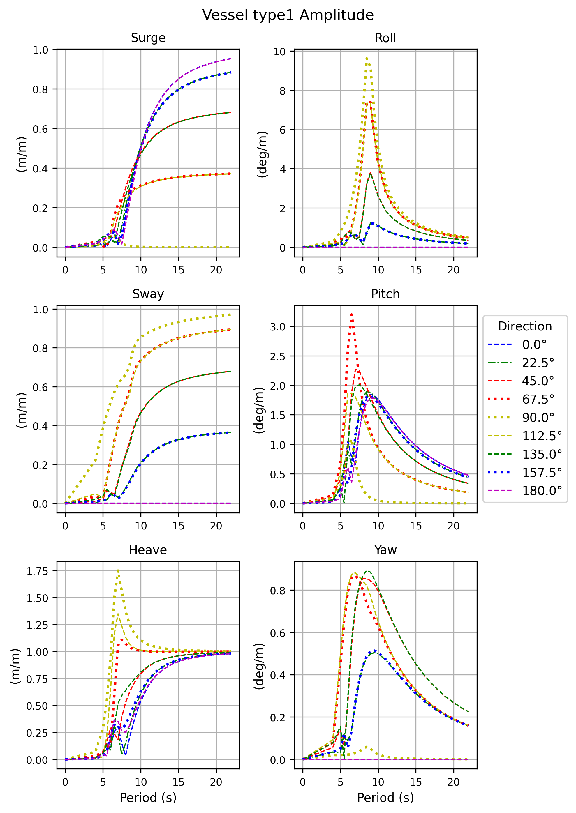
# Create RAO plots (amplitude and phase) and save to the defined folder
model.SaveRAOplots(r'tests\tmptestfiles')
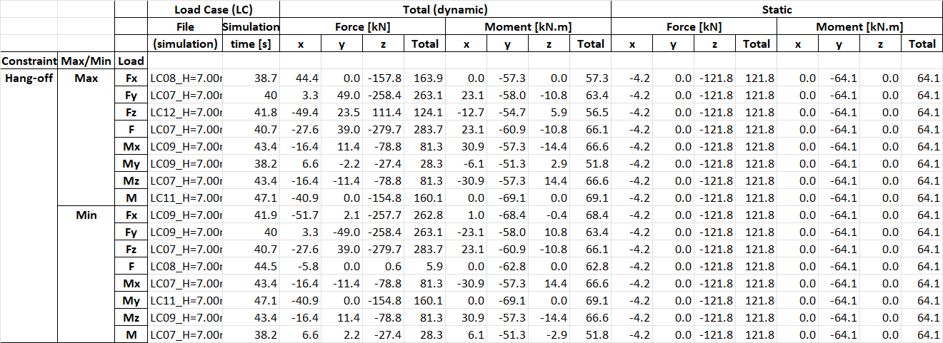
Example 7 - Extract extreme (max. and min.) Constraint loads (force and moment) from multiple simulation files
import NsgOrcFx as ofx

model = ofx.Model()

# create the objects (vessel, constraint, and line)
vessel = model.CreateObject(ofx.ObjectType.Vessel)
constraint = model.CreateObject(ofx.ObjectType.Constraint)
line = model.CreateObject(ofx.ObjectType.Line)

# connect the constraint to the vessel
constraint.name = 'Hang-off'
constraint.InFrameConnection = vessel.name
constraint.InFrameInitialX = 35
constraint.InFrameInitialY = 0
constraint.InFrameInitialZ = -7
constraint.InFrameInitialDeclination = 155 # adjust the nominal top angle

# connect the line End A to the constraint,
# anchor the End B, 155m horizontally away from A,
# and set the line length
line.EndAConnection = constraint.name
line.EndAX, line.EndAY, line.EndAZ = 0, 0, 0
line.EndAxBendingStiffness = ofx.OrcinaInfinity() # to produce moment reaction loads to extract
line.EndBConnection = 'Anchored'
line.PolarReferenceAxes[1] = 'Global Axes'
line.PolarR[1], line.EndBY, line.EndBHeightAboveSeabed = 155, 0, 0
line.Length[0] = 200

# generate the load cases (Example #3)
model.GenerateLoadCases('Dean stream', [135,180,225], [6,7], [9,10], '.')

# run the simulations with multi-threading
ofx.ProcMultiThread('.','.')

# extract extreme loads for the constraint
ofx.ExtremeLoadsFromConstraints('.','.\Results.xlsx')
Example 8 - Generate vessel response for multiple wave directions and Hs x Tp combinations
The method ProcessExtremeResponses also sumarizes the load cases for each wave direction (Hs and Tp combination)
that produces the maximum value for each DOF parameter
# for each wave direction (coming from), define the list with tuples of (Hs, Tp) values
# below is an example with 8 wave directions
# this data is typically obtained from the metocean report
waveDirsHsTp = {
    'N': [
        (4.1,5.1), (4.4,5.6), (4.6,6.1), (4.8,6.5), (5,7), (5.2,7.5), (5.3,7.9),
    ],
    'NE': [
        (5.4,8.4), (5.5,8.9), (5.5,9.3), (5.5,9.8), (5.5,10.3), (5.4,10.7), (5.3,11.2)
    ],
    'E': [
        (5,11.7), (4.9,12.1), (4.6,12.6), (4.3,13.1), (3.9,13.5), (3.5,14), (2.8,14.5)
    ],
    'SE': [
        (5.9,8.5), (6.1,8.9), (6.2,9.4), (6.3,9.9), (6.3,10.3), (6.4,10.8), (6.4,11.3),
    ],
    'S': [
        (4.5,5.2), (4.7,5.6), (4.9,6.1), (5.2,6.6), (5.5,7), (5.6,7.5), (5.7,8),
    ],
    'SW': [
        (6.4,11.7), (6.3,12.2), (6.3,12.7), (6.2,13.1), (6,13.6), (5.7,14.1), (5.6,14.6),
    ],
    'W': [
        (5.2,15), (4.8,15.5), (4.3,16), (3.6,16.4),
    ],
    'NW': [
        (3.1,9), (3.3,9.5), (3.5,10), (3.7,10.4), (3.9,10.9), (4.1,11.4), (4.3,11.8),
    ],
    }

import NsgOrcFx as ofx

# create model and vessel
model = ofx.Model()
vessel = model.CreateObject(ofx.ObjectType.Vessel)
vesselName = vessel.name

# set irregular wave (required for vessel response analysis)
model.environment.WaveType = 'JONSWAP'

# set north direction (required for wave direction definition)
model.general.NorthDirectionDefined = 'Yes'
model.general.NorthDirection = 90

# process extreme responses
model.ProcessExtremeResponses(
    vesselName,
    [35, 0, 0], # position where responses are extracted
    waveDirsHsTp, # wave directions with Hs and Tp values
    r".\tests\tmptestfiles\vessel response.xlsx", # output excel file
    )

# the generated excel file lists the extreme responses for all wave conditions defined above
# and the load cases that lead to the maximum value for each response DOF parameter
# in addition to the results directly provided by OrcaFlex, rotation (vectorial sum of roll and pitch) is included
1 maintainer

Release files for NsgOrcFx 1.0.36
For a detailed explanation of source distributions (sdists) and built distributions (wheels), please see the package formats documentation.
Source distribution (sdist)
| File | Size | Uploaded | |
|---|---|---|---|
| nsgorcfx-1.0.36.tar.gz | 55.2 kB | Details |
Built distribution (wheel)
| File | Interpreter | ABI | Platform | Reset |
|---|---|---|---|---|
| nsgorcfx-1.0.36-py3-none-any.whl | Python 3 | none | any | Details |
Total release size: 109.6 kB
Release files / nsgorcfx-1.0.36.tar.gz
| Download URL | nsgorcfx-1.0.36.tar.gz |
|---|---|
| Size | 55.2 kB |
| Tags | Source |
|
SHA-256 checksum How to use checksums |
b463d08508bce2ec1b15fbb80860cac5835e85d85925670cec01ba8628f98428
|
|
BLAKE2b-256 checksum How to use checksums |
9a0997d9b60a9aa4a138676159c3e7a364f83ea0f9fce87c17ad6b7ee24a4910
|
| Upload date | |
|
Uploaded using Trusted Publishing? What is trusted publishing? |
No |
| Uploaded via |
twine/6.2.0 CPython/3.14.0
|
Release files / nsgorcfx-1.0.36-py3-none-any.whl
| Download URL | nsgorcfx-1.0.36-py3-none-any.whl |
|---|---|
| Size | 54.5 kB |
| Tags | Python 3 |
|
SHA-256 checksum How to use checksums |
19583f16d44ee4937c68fb132ad549bd9404a7df8d1ec4b39c520142ff7e60b5
|
|
BLAKE2b-256 checksum How to use checksums |
f80e5b38bb95e53bbe9175c260cface9024d08c6e993a30301b3e3c798c488fa
|
| Upload date | |
|
Uploaded using Trusted Publishing? What is trusted publishing? |
No |
| Uploaded via |
twine/6.2.0 CPython/3.14.0
|














