
NSS Yield Curve Engine





Fits the U.S. Treasury yield curve every week since 1990 and splits it into the parts people argue about: where the Fed is expected to take rates, the term premium, inflation expectations and recession odds. Each estimate is checked on a simulated market where the answer is known, then against the Federal Reserve's own numbers.



Website · Live dashboard · Results · Methodology · Research note · Changelog
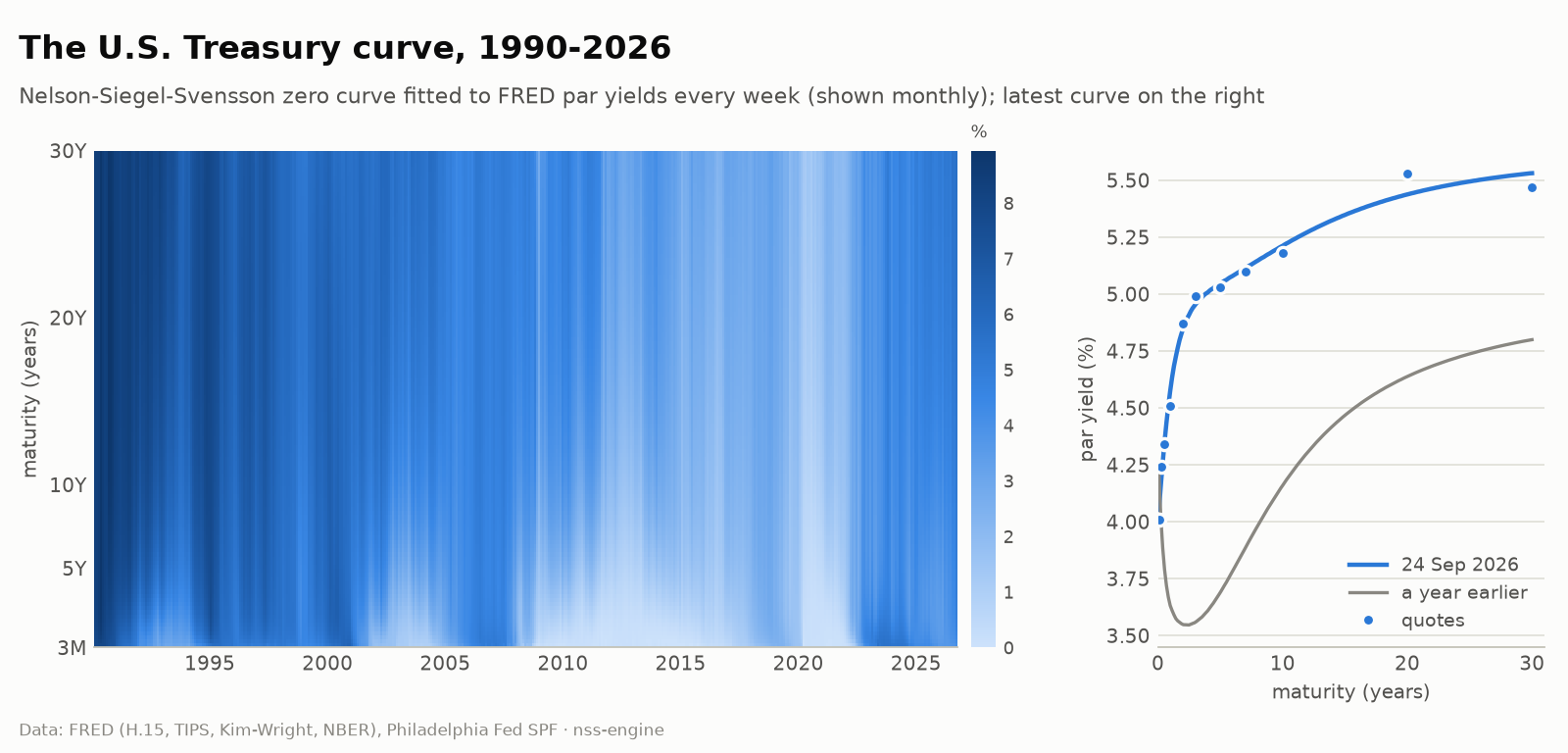
A Nelson–Siegel–Svensson curve fitted to FRED's Treasury yields every week since 1990. The pale stretches are the zero-rate years.
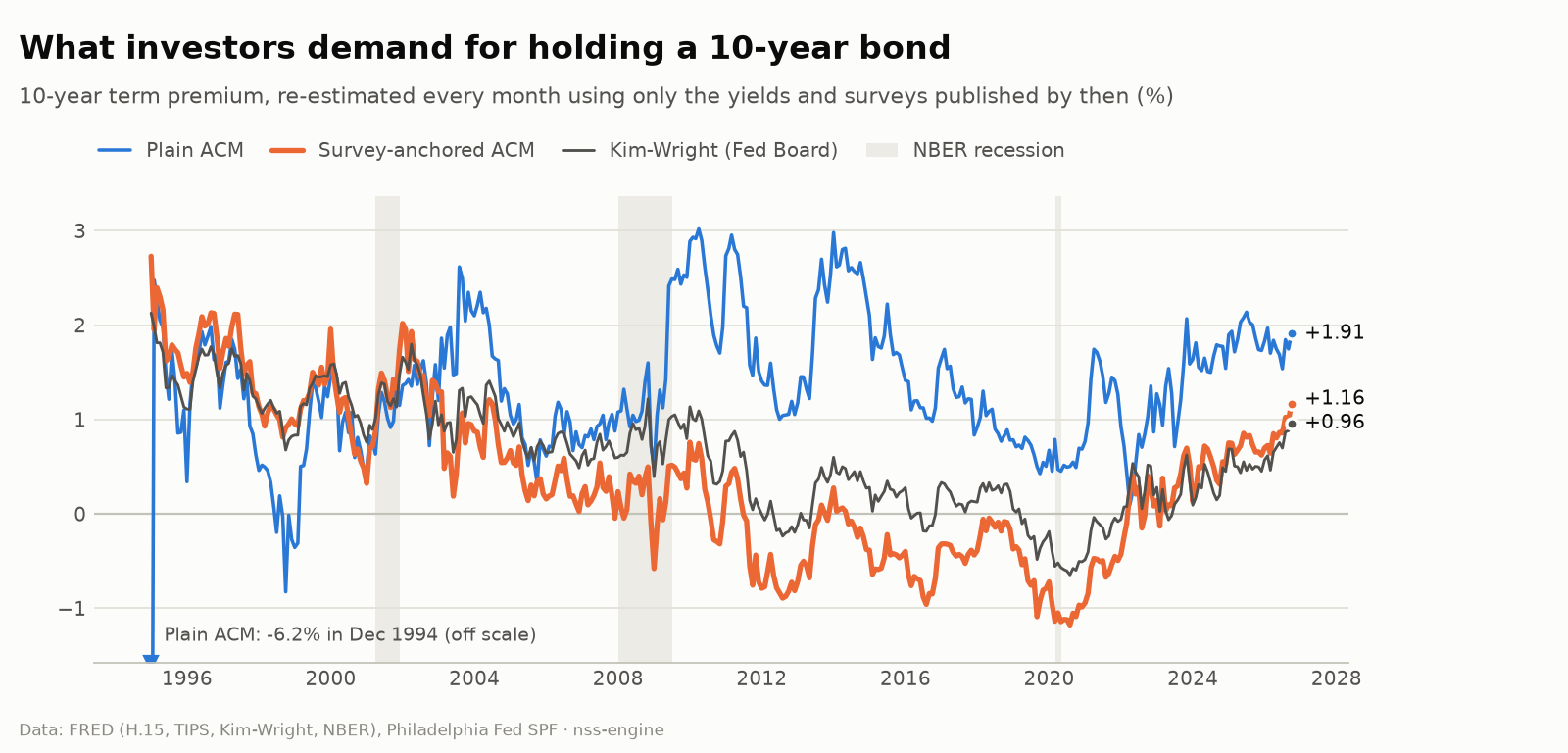
The 10-year term premium as it would have been estimated at each date, using only data published by then. The textbook model (ACM, blue) swings with every re-estimation and sits about a point above the Fed Board's Kim–Wright estimate (grey). Anchoring its expected rates to the Survey of Professional Forecasters (orange) makes it stable and brings it much closer to Kim–Wright. On 24 September 2026: a 5.18% ten-year zero yield = 4.02% expected short rate
- 1.16% term premium.
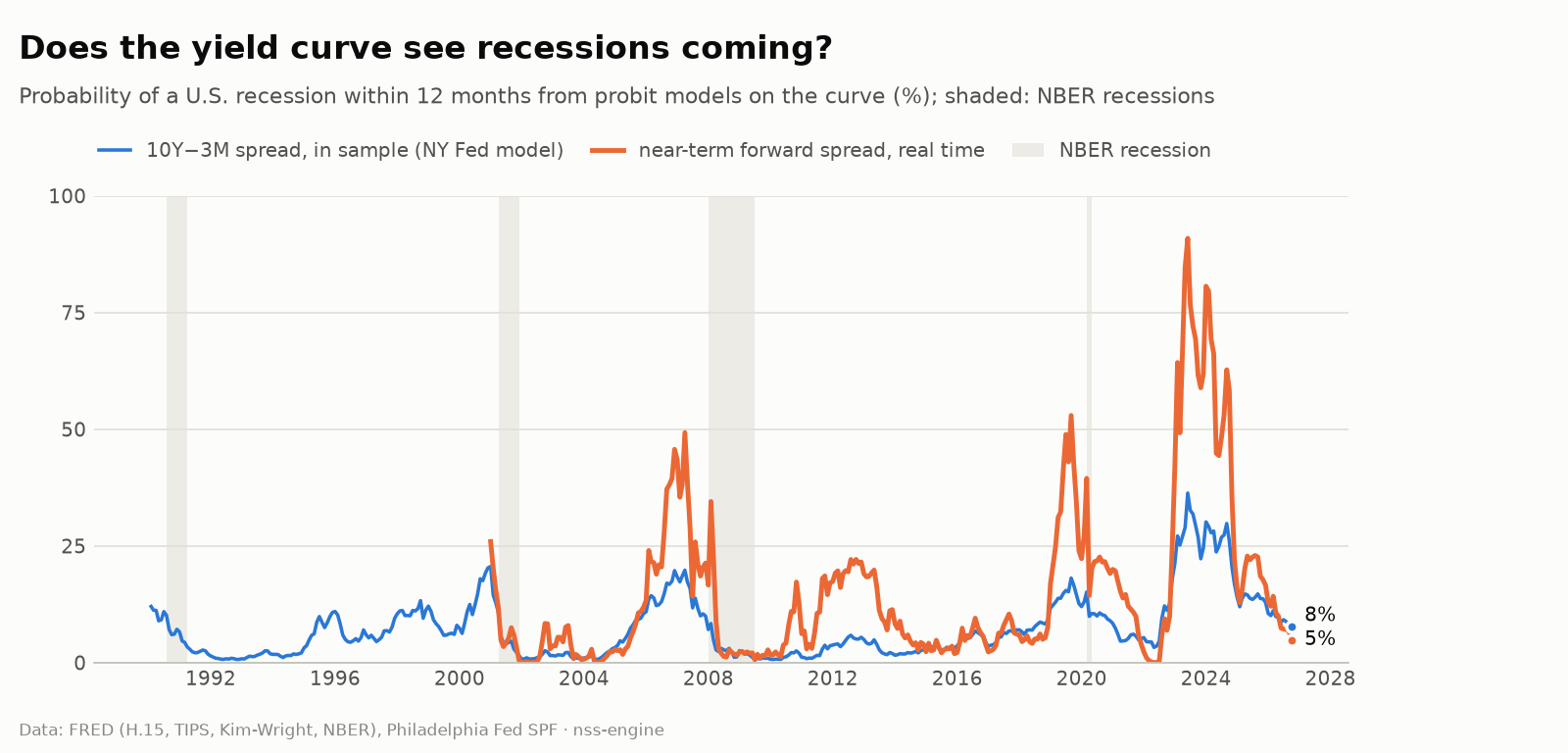
Recession odds from the curve, in sample and in pseudo-real time (only recessions known at each date). The 2022–24 inversion pushed the real-time model to 90% and no recession has followed so far. Four recessions since 1990 are not much to learn from.
Install
pip install nss-engine
nss-engine run          # FRED data since 1990 -> output/dashboard.html, report.md, CSVs
No API key is needed. pip install "nss-engine[surveys]" adds the survey
anchors (it reads the Philadelphia Fed's Excel files), [figures] the PNG
charts. Or run the Colab notebook
in a browser, or nss-engine run --source synthetic offline.
What it finds
From the latest run of the live workflow on FRED data (1990–2026). Details, tables and tests are in docs/results.md.
- Fitting the curve. Median error 3.8 bp over 1,917 weekly curves, and 10.0 bp from the Federal Reserve's own curve, against 16.3 bp the textbook way. FRED's yields are par yields, not the zero rates most Nelson–Siegel code assumes (research note).
- Term premium. The survey-anchored 10-year premium is within 28 bp RMSE of Kim–Wright (plain ACM: 123 bp) and tracks a model-free survey premium best (correlation 0.89). Estimated in real time it agrees 0.91–0.94 with its own full-sample series; plain ACM 0.43–0.70.
- Checked against the source. Run on the Fed's curve since 1961, as its authors do, the engine's ACM code moves one for one with the New York Fed's published term premium (correlation 1.000, a constant 20 bp offset). Starting in 1990 instead adds about 65 bp, which is most of plain ACM's gap to Kim–Wright.
- Bond returns. Plain ACM's real-time premium and the Fama–Bliss forward spread predict one-year returns on the 10-year bond out of sample (R² 8.8% and 7.6%, p ≤ 0.02). The survey-anchored premium does not: the surveys kept expecting rate rises that never came, so it expected bonds to lose to bills while they beat them.
- Breakeven inflation. Against the Fed's own TIPS curve, the engine's
5y5y breakeven is closer (20 bp RMSE) than FRED's published
T5YIFR(27 bp, 9 bp too low on average). On simulated markets it beats FRED's formulas at every maturity. - Recessions. The near-term forward spread beats the classic 10Y−3M spread out of sample (AUC 0.71 vs 0.61), but with three recessions to score, the 90% interval on the gain includes zero.
- Forecasts. Every model loses to "no change" at 1 month (Diebold–Mariano p < 0.001); half model, half random walk only ties it at 6–12 months (p ≥ 0.49).
Several things did not work, and the results page keeps them: robust fitting moves the curve away from the Fed's, bias-corrected VARs make the real-time premium worse, splitting the slope into expectations and term premium (Rosenberg & Maurer) predicts recessions worse than the plain spread since 2005, the Cochrane–Piazzesi bond-return factor does far worse than the historical average out of sample, and the arbitrage-free model's forecast intervals are significantly too wide.
What it does
- Data: FRED's 11 Treasury constant-maturity yields, TIPS real yields, NBER recessions and Kim–Wright; the Fed's GSW nominal and TIPS curves; the New York Fed's ACM term premium; the Philadelphia Fed's SPF. Cached, retried, and read from the cache when a source is down.
- Calibration: NSS fitted to par yields by variable projection, an exhaustive grid over the decay rates and multi-start refinement with an analytic Jacobian, with confidence bands and optional robust fitting. About 26 ms per curve.
- Term premium: Adrian–Crump–Moench, plain or with expectations anchored to surveys (the default) or bias-corrected; full sample and re-estimated month by month; checked against the New York Fed's published series and against the excess returns bonds went on to earn.
- Inflation: TIPS real curve, zero-coupon and 5y5y forward breakevens, compared with FRED and the Fed.
- Recessions: NY Fed-style probit, the near-term forward spread (Engstrom & Sharpe) and expectations vs premium (Rosenberg & Maurer), all scored in pseudo-real time with block-bootstrap intervals.
- Forecasting: Diebold–Li, state-space (Kalman filter, MLE) and arbitrage-free (AFNS) dynamic Nelson–Siegel against the random walk, with Diebold–Mariano and coverage tests.
- Risk and relative value: duration, convexity, key-rate and factor durations, carry and roll-down, rich/cheap z-scores without look-ahead.
- Outputs: interactive dashboard (light/dark), Markdown report, CSV/JSON, PNG charts, shields.io badges, and a website rebuilt from live data every weekday.
As a library
from nss_engine import calibrate_panel, fit_acm, zero_panel
from nss_engine.data import load_treasury_yields, load_spf_bill_forecasts

yields = load_treasury_yields(start="1990-01-01")      # weekly, columns = maturities (years)
fit = calibrate_panel(yields)                          # one NSS curve per week
curve = fit.curve(-1)                                  # the latest curve
curve.zero([2, 10]), curve.forward(5), curve.par_yield(30)

acm = fit_acm(zero_panel(fit.params), surveys=load_spf_bill_forecasts())
acm.decomposition(10).tail()                           # yield = expected short rate + term premium

from nss_engine.data import load_tips_yields
from nss_engine.inflation import breakevens, fit_real_curve
real = fit_real_curve(load_tips_yields())              # TIPS real curve, weekly since 2003
breakevens(fit.params, real.params).tail()             # 5Y, 10Y and 5y5y breakeven inflation

from nss_engine.returns import excess_returns
zeros = zero_panel(fit.params)
excess_returns(zeros).tail()                           # what 2/5/10-year bonds earned over bills
acm.expected_excess_returns().tail()                   # what the model expected them to earn
More in examples/quickstart.py (risk, carry,
uncertainty bands) and the notebook.
How it is tested
Real market data has no "right answer", so every model is first checked on a simulated market with a known truth: a dynamic NSS market for the calibrator, an arbitrage-free affine market with a known term premium and simulated surveys, and a TIPS market with a known breakeven curve. Then it is checked against independent estimates on real data: the Fed's curves, Kim–Wright, FRED's breakevens.
- Unit, property-based (Hypothesis) and statistical tests on Python 3.10–3.13,
Linux and Windows, pandas 2 and 3, with
ruffandmypy. - Math identities (forward curves integrate to zero curves, par bonds price at 100, key-rate durations sum to duration), a brute-force check of the calibrator's global optimum, Jacobians against finite differences, and Kalman filters against a textbook implementation.
- No look-ahead: scrambling every outcome, yield or survey published after a date leaves that date's real-time estimate unchanged.
How the calibration works
For fixed decay rates the NSS model is linear in its four betas, so the six-parameter fit becomes a two-dimensional search: closed-form betas for any $(\lambda_1, \lambda_2)$, an exhaustive grid over that plane to find every basin, then a local par-yield refinement from each basin with an analytic gradient. Constraints keep the two humps apart and inside the quoted maturities; a week-to-week penalty on the decay rates, tuned against the true curve on simulated data, keeps the parameters stable. Details, derivations and every other model are in docs/methodology.md.
Limitations
- Constant-maturity yields are interpolated on-the-run par yields, not prices of individual bonds: residuals are a curve-shape signal, not tradeable mispricings.
- The term premium depends on the model; survey anchors help only as far as the surveys are right. Breakevens include risk and liquidity premia.
- Four recessions since 1990 are too few to be sure which signal is best, and the 2022–24 inversion has not been followed by a recession.
- Forecast intervals ignore parameter uncertainty and model misspecification.
Background
This started as a sophomore-year script: a Nelson–Siegel fit to FRED data with a 3-D Plotly surface. 1.0 rebuilt it; 2.0 fitted the quotes as what they are (par yields) and checked the result against the Federal Reserve; 2.1 put error bars on the headline claims and withdrew one; 2.2 added the term premium and arbitrage-free dynamics; 2.3 survey anchors and significance tests; 2.4 breakeven inflation and this website; 2.5 the check against the New York Fed's series and against realized bond returns. The CHANGELOG lists what was wrong in each version and how it was fixed.
If you use it, please cite it (CITATION.cff). References are in docs/methodology.md.
Data: Board of Governors of the Federal Reserve System (H.15, GSW curves, Kim–Wright), via FRED (Federal Reserve Bank of St. Louis); Federal Reserve Bank of Philadelphia (Survey of Professional Forecasters); NBER. MIT license. Educational project, not investment advice.
1 maintainer

Metadata
1 maintainer
Release files for nss-engine 2.5.1
For a detailed explanation of source distributions (sdists) and built distributions (wheels), please see the package formats documentation.
Source distribution (sdist)
| File | Size | Uploaded | |
|---|---|---|---|
| nss_engine-2.5.1.tar.gz | 1.1 MB | Details |
Built distribution (wheel)
| File | Interpreter | ABI | Platform | Reset |
|---|---|---|---|---|
| nss_engine-2.5.1-py3-none-any.whl | Python 3 | none | any | Details |
Total release size: 1.3 MB
Release files / nss_engine-2.5.1.tar.gz
| Download URL | nss_engine-2.5.1.tar.gz |
|---|---|
| Size | 1.1 MB |
| Tags | Source |
|
SHA-256 checksum How to use checksums |
8cc802b9455df5b399c176db1af16fc28a1db9567c0082d9cc4d6bbe3500d6fe
|
|
BLAKE2b-256 checksum How to use checksums |
05e6498aa8a0ca364043b3efaf5dfac00c242ecf434abd61ed74281561a57d51
|
| Upload date | |
|
Uploaded using Trusted Publishing? What is trusted publishing? |
Yes |
| Uploaded via |
twine/7.0.0 CPython/3.13.14
|
Provenance
Provenance describes where a file came from. On PyPI, provenance is shared via attestations, which provide a verifiable record of the build or publishing details. View details, limitations and caveats.


PyPI Publish Attestation
PyPI verified that this artifact, at this checksum, originated from the publisher listed below.
Signed by GitHub Actions, verified by PyPI on Oct 2, 2026.
Transparency logRelease files / nss_engine-2.5.1-py3-none-any.whl
| Download URL | nss_engine-2.5.1-py3-none-any.whl |
|---|---|
| Size | 136.7 kB |
| Tags | Python 3 |
|
SHA-256 checksum How to use checksums |
3f56bc05938cce5aefb9245f0ddd44d76a0a0968c6671f81516e3405df222fe6
|
|
BLAKE2b-256 checksum How to use checksums |
4ad26e47804709c3984ccdb08b28e12afe648a608b09e971fb4358fbd559aaae
|
| Upload date | |
|
Uploaded using Trusted Publishing? What is trusted publishing? |
Yes |
| Uploaded via |
twine/7.0.0 CPython/3.13.14
|
Provenance
Provenance describes where a file came from. On PyPI, provenance is shared via attestations, which provide a verifiable record of the build or publishing details. View details, limitations and caveats.
PyPI Publish Attestation
PyPI verified that this artifact, at this checksum, originated from the publisher listed below.
Signed by GitHub Actions, verified by PyPI on Oct 2, 2026.
Transparency log













