
MCMC plotting framework for official results from neutrino oscillation experiments


Project description
NuMCMCTools


This package is intended as a lightweight tool to assist in analysis using public releases of MCMC chains from neutrino oscillation analyses. The following experiments have released data compatible with this software:
- T2K collaboration: arXiv:2506.05889 (2025), DATA RELEASE
- NOvA collaboration: Phys. Rev. D 106, 032004 (2022), DATA RELEASE
Installation
To install numcmctools with PyPI, run the following command:
pip install numcmctools
To install directly from source, first clone numcmctools with git:
git clone https://github.com/NuMCMCTools/NuMCMCTools.git
enter the new NuMCMCTool directory and simply run:
pip install .
The pacakge does not need to be installed to use it, you can simply git clone
the package and add your own macros that include the numcmcmtools folder.
File Format
MCMC samples
The expected input format for this code is a ROOT file containing at least one TTree. The tree can have any name. Inside the tree, there will be at least six branches called:
- DeltaCP, in radians, across any $2\pi$ interval
- Theta13, in radians, [0, $\pi$/2]
- Theta23, in radians, [0, $\pi$/2]
- Theta12, in radians, [0, $\pi$/2]
- Deltam2_32, in $\text{eV}^2$
- Deltam2_21, in $\text{eV}^2$
which correspond to the standard parameters of neutrino mixing; the first four are the PMNS angles, and the last two are the mass splittings. For more information on the parameterization see the PDG review on neutrino mixing.
Priors
Each parameter has some prior set by the original analyzers. The format of this
information is a TList object named priors, containing a TNamed for each
branch, which specifies the name of the branch and its prior.
The priors are specified as:
UniformGaussian(mean, sigma)BimodalGaussian(mean1, sigma1, mean2, sigma2, bias)where bias is in % and optional, default 50%.Step(bias, boundary)where bias is in % and boundary is optional, default 0
There is then a further specification as to which variable the functional form applies to. For example, a specification of
Theta23 Uniform:sin^2(Theta23)
indicates that the prior for Theta23 is uniform in $\sin^2\theta_{23}$.
Empirical priors
Optionally, file can contain 1D or 2D empirical priors to be applied by default to the plots when the empirical_priors object input to add_plot function is set to None. For this, there needs to be a TDirectoryFile object named empirical_priors. Each empirical prior object inside that directory can be either TGraph2D or THnD. Additionally, a TList named priors needs to contain, a detailed metadata for each external empirical prior. The TNamed entry inside of TList must be in a format:
- Name: unique name that matches
TNamedinside ofTList - Title:
EmpiricalPriorprefix, to distinguish this from the standard functional priors. - Title: parameter names separated by colon, e.g.
sin^2(2Theta13):abs(Deltam2_32) - Title: Optional string "NO" for empirical priors only applied to Normal Mass Ordering, IO for the Inverted mass ordering, or none for an empirical prior applied across both Mass Orderings.
- Title: 1 if the empirical prior should be applied automatically, or 0 if not.
Example:
DayaBay2D_2024_IOEmpiricalPrior:sin^2(2Theta13):abs(Deltam2_32):IO:1for a 2D constraint automatically applied in the Inverted Mass Orderingsome_constraint_from_theoryEmpiricalPrior:sin^2(2Theta13):sin^2(Theta23):1for a 2D constraint automatically applied across both mass orderings.
The unique names for the empirical priors inside the priors TList must match the name of the THnD or TGraph2D inside of the empirical_priors TDirectory. Example provided in examples/testchaindata.root
Other
The file additionally contains a citation to the original analysis that
produced the chain. The citation must be inside of a TObjString object named
citation.
There may be additional information contained in the file; please see the data release from the particular analysis for more detail.
In this code, the class mcmcsamples is responsible for loading
in the required information from the file. The constructor takes the
filepath for the input file and the name of the oscillation parameters
tree, and an optional argument for additional variables to be loaded.
An example tree (examples/testchaindata.root) with the required
features is provided for testing the functionality of this software.
A very basic script for loading the example tree is
examples/load_mcmc.py and can be run as follows:
python -m examples.load_mcmc
Posterior Density Functions and Contours
After the tree is loaded, an instance of plotstack can be created,
which is initialized with an mcmcsamples instance. Individual
plots can be added to the plot stack. One and two dimensional plots
are currently supported.
A plot is added to the plot stack with the add_plot function, which
takes as arguments an array of the name(s) of the variables to be
plotted as strings, any change in priors to be applied (see section below for details),
the bins and axis ranges for the plots, as defined in
numpy.histogram
or
numpy.histogram2d,
and finally whether to treat the two mass orderings separately
(True) or together (False, default).
Any number of plots can be added to the stack. When all plots are
created, they can be filled by calling fill_plots, which has two
optional arguments. The first causes only the first
n_steps to be filled from the tree; this is useful in testing the
plot stack for very large input trees; the second restricts the number
of steps read from the tree to be batchsize at any given time, which
is helpful for memory management. Above a batch size of approximately
100000, there is no performance impact on the time it takes to read
large trees and fill plots; this value is therefore set at the
default. The number of plots to be filled does have an impact on the run
time of the code.
After the histograms are filled, they are normalized to create probability density functions, such that individual bins are normalized to the width/area of the bin and the integral is normalized to 1.
Credible intervals can be created by calling make_intervals
on either the plot stack or individual plots within the stack. The
function takes an array of credible interval levels.
PDFs and intervals can be drawn with draw_plot and draw_interval
respectively, and can take an Figure argument from matplotlib. When
dividing a figure into subfigures, use the subfigures command, rather
than subplots, as subplots is used internally.
The plot stack can also be used to automatically draw all of the plots in the stack, choosing the optimal dimensions for the subfigure array.
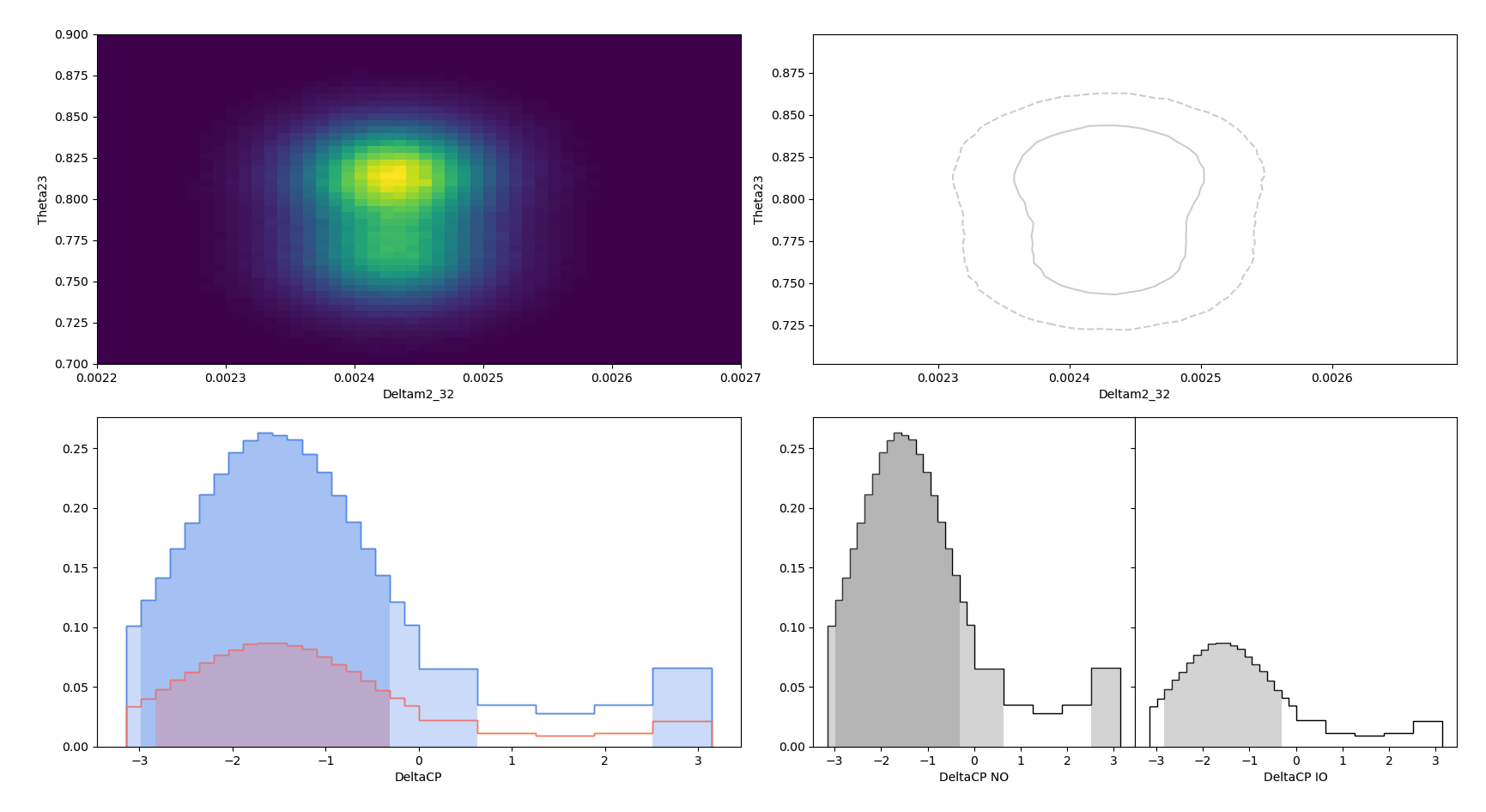
An example of the plotting features is in examples/simpleplots.py and
can be run as follows:
python -m examples.simpleplots
The output of this example should look as follows
Derived Variables
Variables derived from the six required parameters—for example, $\sin^2\theta_{23}$-can be defined and used for plotting. Each new variable must be given a unique name and defined as a function which uses the required parameters as input variables, spelled exactly as they are defined above.
The new variable is then attached to an instance of the mcmcsamples
class using the add_variable function, which takes as arguments the
name of the new variable and the function defining it.
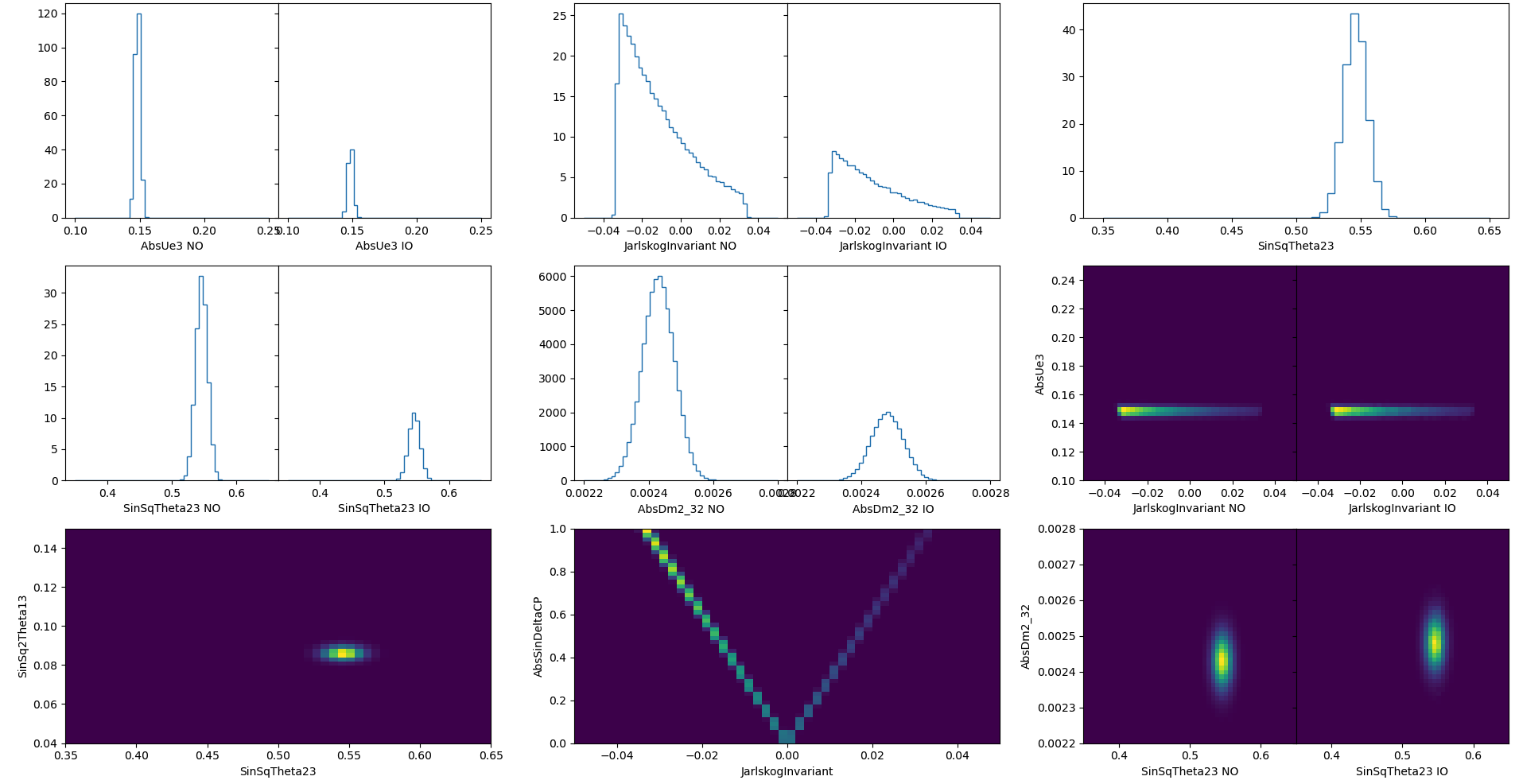
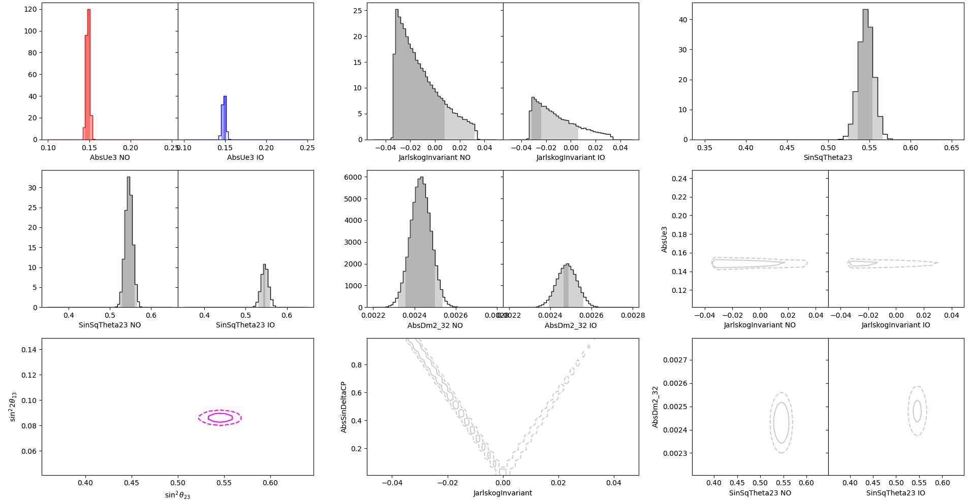
An example of this feature is in examples/custom_variables.py and
can be run as follows:
python -m examples.custom_variables
The output of this example should have two canvases which look as follows
Changing Priors
Priors for parameters can be changed automatically when making plots.
A list of new priors is passed when adding a new plot to the plotstack.
This feature currently only works in 1D and with Uniform or Gaussian priors
in a limited set of transformations of variables. The list of currently
available transformations is:
x
sin(x)
sin^2(x)
cos(x)
cos^2(x)
cos^4(x)
2x
sin(2x)
sin^2(2x)
cos(2x)
cos^2(2x)
cos^4(2x)
exp(-ix)
exp(ix)
abs(ix)
For example, an input chain that has a prior set to be uniform in DeltaCP can have the following passed to the input chain to make plots with a prior uniform in $\sin\delta_{CP}$:
["Uniform:sin(DeltaCP)"]
Examples of this in practice are in the custom_variables example.
Plotting
Plots can be drawn directly from the plotstack (shown in the custom_variables
example), where the arrangement of pdfs or intervals is done algorithmically.
For more control, the figure and its subdivisions can be arranged by the user
and each plot drawn individually. An example of the latter is shown in both the
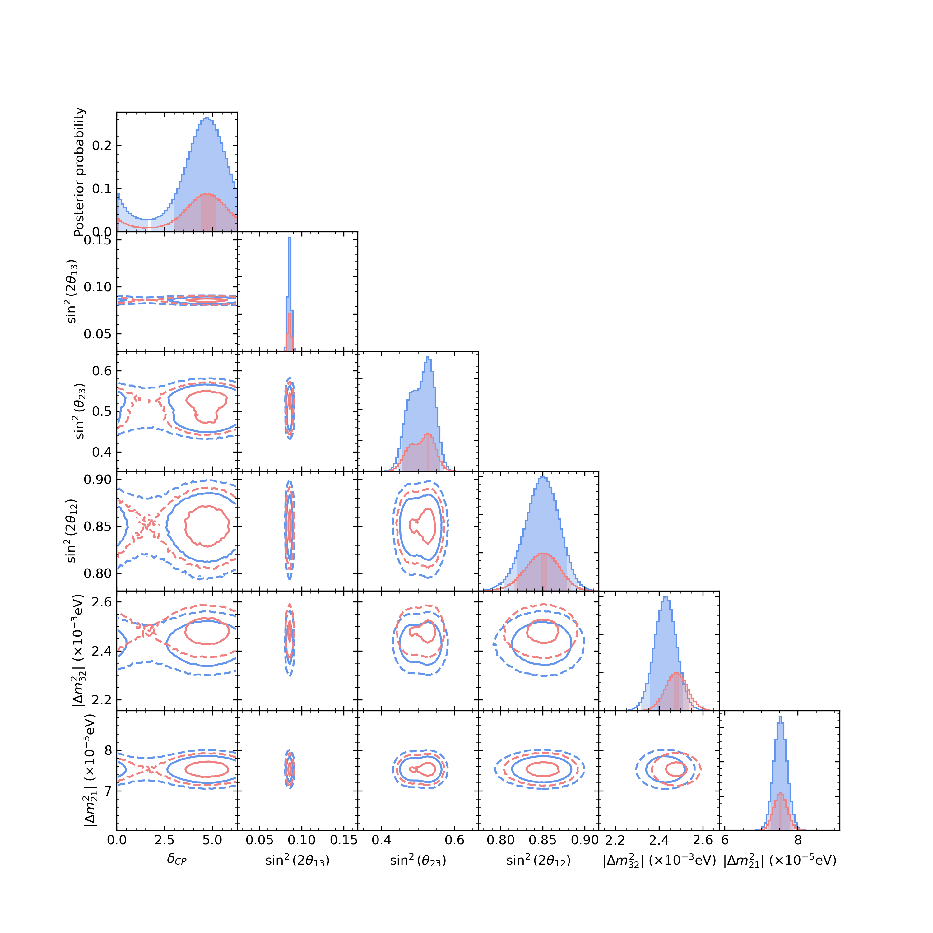
simpleplots example, and in the plot_triangle example, which creates a standard
triangle (corner) plot with the mass ordering separated. This example can be run as
follows:
python -m examples.plot_triangle -f examples/testchaindata.root -c mcmc
or
plot_triangle -f examples/testchaindata.root -c mcmc
if installed throgh pip, which produces the output below.
Release history Release notifications | RSS feed


Download files
Download the file for your platform. If you're not sure which to choose, learn more about installing packages.
Source Distribution
Built Distribution
Filter files by name, interpreter, ABI, and platform.
If you're not sure about the file name format, learn more about wheel file names.
Copy a direct link to the current filters
File details
Details for the file numcmctools-1.1.0.tar.gz.
File metadata
- Download URL: numcmctools-1.1.0.tar.gz
- Upload date:
- Size: 30.2 MB
- Tags: Source
- Uploaded using Trusted Publishing? No
- Uploaded via: twine/6.2.0 CPython/3.12.10
File hashes
| Algorithm | Hash digest | |
|---|---|---|
| SHA256 |
d6a4d4caf5efd1f59e6c2837f5f09770ab6677c90053782f6a0c4e74f2fa9ce1
|
|
| MD5 |
70dfcc44b548a4eb9a69ec9bf9d3ae93
|
|
| BLAKE2b-256 |
aa47818dc3f6192f759a5672fa43e1a32e2bbf76a60569f470f57f518ae49e5e
|
File details
Details for the file numcmctools-1.1.0-py3-none-any.whl.
File metadata
- Download URL: numcmctools-1.1.0-py3-none-any.whl
- Upload date:
- Size: 30.2 MB
- Tags: Python 3
- Uploaded using Trusted Publishing? No
- Uploaded via: twine/6.2.0 CPython/3.12.10
File hashes
| Algorithm | Hash digest | |
|---|---|---|
| SHA256 |
9315f741ed477175b038aa4d17e95920cc29278308fe1ddeacefca3a6283b884
|
|
| MD5 |
01ab75b01db8e70ea7976f52e5ee20ce
|
|
| BLAKE2b-256 |
41090a7a82431016bfb0f7d65b2c4494ef8fa2f5684e734b41fb94f81603054b
|






