
Exact two-, three- and four-flavor neutrino oscillation probabilities for arbitrary time-independent Hamiltonians
Verified details
These details have been verified by PyPIProject links
GitHub Statistics
Maintainers

Project description










NuOscProbExact
Code to compute exact two-, three- and four-neutrino oscillation probabilities using SU(2), SU(3) and SU(4) expansions
Note: The oscillation probabilities are computed exactly, with no approximation beyond floating-point round-off. A regression test suite lives in
tests/and can be run withpytest, and the results are cross-checked against nuSQuIDS, an independent external code — see notebook 17.
What you can compute
Every figure below is produced by a notebook in notebooks/, and the link under each one goes to the code that drew it. The documentation collects the same material, with runnable snippets, on its numerical recipes page.
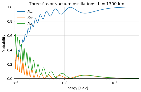 Oscillation probabilities against baseline or energy, for two, three or four flavors. notebook 02 |
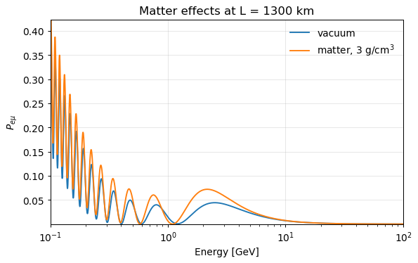 Matter, NSI and Lorentz-invariance violation — each just a different Hermitian matrix. notebook 03 |
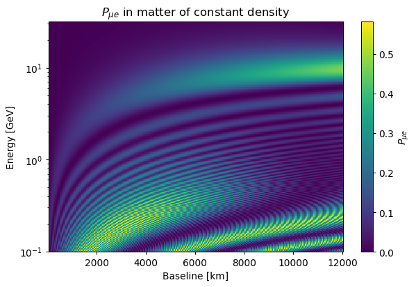 Oscillograms over energy and baseline: 57 600 probabilities in a single call. notebook 04 |
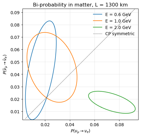 CP violation, as bi-probability ellipses in vacuum and in matter. notebook 05 |
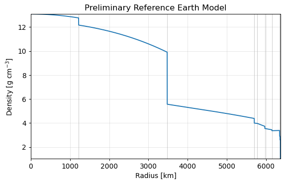 The Earth's density, from the Preliminary Reference Earth Model. notebook 06 |
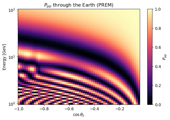 Neutrinos through the Earth, in energy and zenith angle, or between two named sites. notebook 07 |
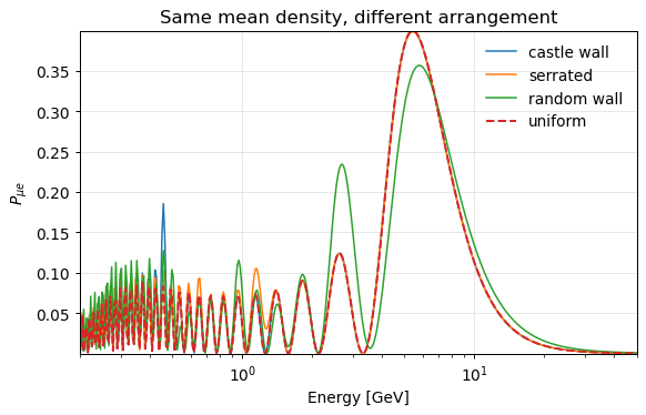 Arbitrary matter profiles — castle walls and worse, exactly. notebook 08 |
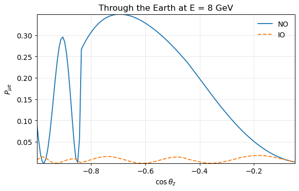 Mass ordering and the θ₂₃ octant, separated by matter through the Earth. notebook 12 |
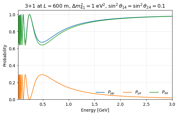 Four flavors: a 3+1 sterile state, resolved at a short baseline. notebook 16 |
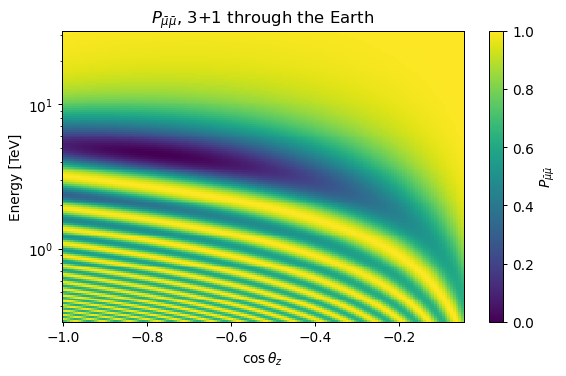 The sterile matter resonance through the Earth, in energy and zenith angle. notebook 16 |
Contents
What is NuOscProbExact?
NuOscProbExact is a Python implementation of the method developed by Ohlsson & Snellman to compute exact neutrino oscillation probabilities for arbitrary time-independent Hamiltonians. The method was revisited and the code presented in the paper NuOscProbExact: a general-purpose code to compute exact two-flavor and three-flavor neutrino oscillation probabilities (arXiv:1904.12391), by Mauricio Bustamante.
The paper covers two and three flavors; the code has since been extended to four, through the SU(4) algebra, which brings 3+1 sterile scenarios into scope. Four is where the closed form ends — see why.
The method relies on expansions of the Hamiltonian and time-evolution operators in terms of SU(2), SU(3) and SU(4) matrices in order to obtain concise, analytical, and exact expressions for the probabilities, that are also easy to implement and evaluate. For details of the method, see the paper above; the four-flavor extension is documented in the methodology page.
What it does
- Exact probabilities for any Hermitian 2×2, 3×3 or 4×4 Hamiltonian. There is no approximation beyond floating-point round-off, and the probabilities agree with the independently written nuSQuIDS to round-off once conventions are matched (notebook 17). Oscillations in vacuum, in matter, with non-standard interactions, in a Lorentz invariance-violating background and with sterile states are not special cases in the code — each is a different matrix handed to the same routine.
- Four flavors, for 3+1 sterile scenarios.
oscprob4nucarries the same closed-form treatment to SU(4), which is the last place it reaches: at five flavors the eigenvalues stop being expressible in radicals, and that is a theorem rather than a missing feature. A 3+1 system is closed and unitary over all four states, so it sits squarely inside the method's assumptions rather than "leaking" out of a three-flavor block. - The evolution operator itself, not only the probabilities, so it can be composed across segments or used to propagate a density matrix.
- Whole scans in one call. Every core routine accepts a stack of Hamiltonians, an array of baselines, or both broadcast against each other, which is tens of times faster than the equivalent Python loop and gives identical results.
- Piecewise-constant matter.
slabspropagates across a sequence of adjacent slabs of arbitrary width and density, solving each exactly and multiplying the operators, at two, three or four flavors. - The Earth.
earthbuilds those slabs from the Preliminary Reference Earth Model, and computes probabilities along a given zenith angle or between two of fifteen predefined locations. A 3+1 crossing is included: the sterile state does not feel the neutral-current potential, so that potential stops cancelling andearthbuilds it per slab. - An optional compiled backend. With
numbainstalled, large batched calls run on compiled kernels; without it the NumPy path is used and the answers are the same to round-off.
What it does not do
- Hamiltonians that vary continuously along the trajectory. See When to use Magnus instead below — this is the one case where a different tool is the right answer, and it is worth knowing before you start.
- More than four flavors. The expansions run to SU(4) and stop, because the closed form does: solving for the eigenvalues means solving the characteristic polynomial in radicals, and at degree five Abel–Ruffini says that cannot be done. Four flavors covers 3+1, which is the case people actually ask for.
- Neutrino production, cross sections, fluxes or detector response. This computes oscillation probabilities and nothing downstream of them.
- Fitting or statistics. There is no likelihood machinery here; the probabilities are meant to be handed to whatever does that.
When to use Magnus instead
NuOscProbExact assumes the Hamiltonian is constant, or piecewise constant. Everything it is good at follows from that — and so does the one case where it is the wrong tool.
Use Magnus instead when the Hamiltonian varies continuously and appreciably over an oscillation length. A smoothly varying profile can always be approximated by slabs, but then the step size is set by the oscillation rather than by the density, and the slab count grows until the calculation is neither exact nor quick.
| Situation | Use | Because |
|---|---|---|
| Constant density | NuOscProbExact | One closed form, no integration |
| Piecewise constant, tens of layers — the Earth through PREM | NuOscProbExact (slabs, earth) |
Each layer solved exactly, operators multiplied |
| Smoothly varying, slow against the oscillation | either | Slabbing converges quickly |
| Smoothly varying, fast against the oscillation — the Sun, adiabatic MSW | Magnus | Slabbing needs ~104 steps per resonance crossing |
| Open systems: decay, decoherence | neither | Needs a Lindblad solver, not a unitary one |
Notebook 14 works the solar case through and shows exactly where the wall is, rather than asserting it.
NuOscProbExact was developed by Mauricio Bustamante. If you use it in your work, please follow the directions on Citing.
Requirements
NuOscProbExact is fully written in Python 3. It uses standard modules that are available, sometimes by default, as part of most Python installations, either stand-alone or via Anaconda. Where a row names an extra, that is the one to install; the rest need nothing beyond numpy. The commands are under Installation below, and are not repeated here.
| To do this | You need | Extra |
|---|---|---|
Compute probabilities (oscprob2nu.py, oscprob3nu.py, oscprob4nu.py) |
numpy, cmath |
— |
Use the bundled sample Hamiltonians (hamiltonians2nu.py, hamiltonians3nu.py, hamiltonians4nu.py) |
numpy, cmath, copy |
— |
Propagate through layered matter or the Earth (slabs.py, earth.py) |
numpy |
— |
| Go faster on large scans (optional) | numba |
fast |
Run the notebooks (notebooks/) |
matplotlib, Jupyter |
notebooks |
Run the regression suite (tests/) |
pytest, scipy, coverage, pytest-cov |
test |
| Build the documentation | Sphinx and friends | docs |
Only numpy is ever required. scipy is used by the test suite alone, to cross-check the evolution operator against an independent matrix exponential; the library itself never imports it. numba is entirely optional — it is worth roughly 1.5x to 20x on large scans, depending on their size and the number of flavors, and without it the NumPy path is used and the results are identical to round-off.
Installation
NuOscProbExact is pure Python: there is nothing to compile or link.
Python version: The code requires Python 3.9 or newer, and every release is tested on 3.9, 3.10, 3.11, 3.12, and 3.13. The floor comes from
numpy.broadcast_shapes, which the batched paths use and which arrived in NumPy 1.20; 3.9 is also the oldest version for which the optionalnumbabackend still has a wheel.
From PyPI (recommended)
pip install nuoscprobexact
That is the whole installation. The only required dependency is numpy.
The optional extras add what each task needs, and can be combined:
pip install "nuoscprobexact[fast]"       # numba, for the compiled batched kernels
pip install "nuoscprobexact[notebooks]"  # Jupyter, matplotlib and scipy, for notebooks/
pip install "nuoscprobexact[test]"       # pytest, scipy and coverage, to run the suite
pip install "nuoscprobexact[docs]"       # Sphinx and friends, to build the documentation
Then, in your own code:
import numpy as np
import oscprob3nu
import hamiltonians3nu
import globaldefs as gd

h_vacuum = hamiltonians3nu.hamiltonian_3nu_vacuum_energy_independent(
    gd.S12_NO_BF, gd.S23_NO_BF, gd.S13_NO_BF, gd.DCP_NO_BF,
    gd.D21_NO_BF, gd.D31_NO_BF)

prob = oscprob3nu.probabilities_3nu(
    np.asarray(h_vacuum)/1.e9, 1300.0*gd.CONV_KM_TO_INV_EV)
The modules are installed under their bare names --- oscprob2nu, oscprob3nu, oscprob4nu, hamiltonians2nu, hamiltonians3nu, hamiltonians4nu, globaldefs, fastkernels, slabs, earth --- which is the same way the paper and the worked examples refer to them.
From GitHub
Install from a clone if you want the notebooks, the worked examples from the paper, the regression suite, or a version that is not yet released:
git clone https://github.com/mbustama/NuOscProbExact.git
cd NuOscProbExact
pip install -e .
-e installs in editable mode, so edits to src/ take effect without reinstalling. The extras work the same way, for example pip install -e ".[fast,test]".
A clone gives you the following file structure:
NuOscProbExact/
├── .github/                         # Continuous integration (GitHub Actions)
│   └── workflows/
│       ├── tests.yml                # The suite: five Pythons, all three backends
│       ├── lint.yml                 # ruff, and the docs build under -W
│       ├── pages.yml                # Builds and deploys the docs to GitHub Pages
│       └── publish.yml              # Publishes to PyPI on a GitHub Release
├── .gitignore                       # Build, cache, and generated-output artefacts
├── CHANGELOG.md                     # Notable changes, rendered as a docs page
├── LICENSE                          # MIT license
├── README.md                        # Project overview and worked examples
├── pyproject.toml                   # Packaging metadata and pytest configuration
├── examples/                        # Runnable scripts, one per scenario, linked from README.md
│   ├── example_2nu_trivial.py       # Two-flavor, arbitrary Hamiltonian
│   ├── example_2nu_vacuum.py        # Two-flavor, oscillations in vacuum
│   ├── example_2nu_vacuum_coeffs.py # Two-flavor, expansion coefficients
│   ├── example_3nu_trivial.py       # Three-flavor, arbitrary Hamiltonian
│   ├── example_3nu_vacuum.py        # Three-flavor, oscillations in vacuum
│   ├── example_3nu_vacuum_coeffs.py # Three-flavor, expansion coefficients
│   ├── example_3nu_matter.py        # Three-flavor, oscillations in matter
│   ├── example_3nu_nsi.py           # Three-flavor, matter with NSI
│   └── example_3nu_liv.py           # Three-flavor, LIV background
├── docs/                            # Sphinx documentation
│   ├── Makefile                     # `make html` on Linux and macOS
│   ├── make.bat                     # `make html` on Windows
│   ├── requirements.txt             # Documentation-only dependencies
│   └── source/
│       ├── conf.py                  # Sphinx configuration
│       ├── index.rst                # Landing page
│       ├── installation.rst         # Requirements, installation, file tree
│       ├── quickstart.rst           # Shortest path to a probability
│       ├── recipes.rst              # Numerical recipes, with pre-generated figures
│       ├── methodology.rst          # The SU(2), SU(3) and SU(4) expansions
│       ├── functions.rst            # API reference, from the docstrings
│       ├── references.rst           # Bibliography
│       ├── refs.bib                 # BibTeX entries for the bibliography
│       ├── changelog.rst            # Includes the root CHANGELOG.md
│       └── _static/
│           ├── nuoscprobexact_logo.png
│           └── slabs_composition.svg  # How slabs compose, drawn for quickstart.rst
├── img/                             # Figures from earlier versions of README.md
│   ├── prob_3nu_vacuum_vs_baseline_ee_em_et.png
│   ├── prob_3nu_vacuum_vs_energy_ee_em_et.png
│   └── gallery/                     # Figures lifted from the notebooks, shown in README.md
│       ├── gallery_biprobability.png
│       ├── gallery_earth.png
│       ├── gallery_matter.png
│       ├── gallery_ordering.png
│       ├── gallery_oscillogram.png
│       ├── gallery_prem.png
│       ├── gallery_profiles.png
│       ├── gallery_sterile.png
│       ├── gallery_sterile_earth.png
│       └── gallery_vacuum.png
├── notebooks/                       # Worked examples, with their figures stored inline
│   ├── 01_basics.ipynb              # Units, one probability, and broadcasting
│   ├── 02_vacuum_oscillations.ipynb # Against baseline and against energy
│   ├── 03_matter_nsi_liv.ipynb      # Constant-density matter, NSI, and LIV
│   ├── 04_oscillogram.ipynb         # Energy-baseline maps in one call
│   ├── 05_biprobability.ipynb       # CP ellipses, in vacuum and in matter
│   ├── 06_earth_and_prem.ipynb      # PREM, chord geometry, and slabs
│   ├── 07_earth_probabilities.ipynb # Through the Earth, and between sites
│   ├── 08_unusual_density_profiles.ipynb  # Castle-wall and other hand-built profiles
│   ├── 09_performance.ipynb         # Looping vs broadcasting, and the backend
│   ├── 10_paper_figures.ipynb       # The two figures from arXiv:1904.12391
│   ├── 11_exact_vs_approximations.ipynb  # Where the textbook formulas break down
│   ├── 12_ordering_and_octant.ipynb # Normal vs inverted, and the 23 octant
│   ├── 13_antineutrinos.ipynb       # Conjugate and flip, and two ways to slip
│   ├── 14_solar_and_adiabatic_msw.ipynb  # The MSW resonance, and the cost wall
│   ├── 15_numerical_edge_cases.ipynb  # Degeneracies, and what does not go NaN
│   ├── 16_four_neutrinos.ipynb      # A 3+1 sterile state, through the SU(4) expansion
│   ├── 17_cross_checks.ipynb        # Corroboration from nuSQuIDS and Zaglauer-Schwarzer
│   ├── 18_evolution_operator.ipynb  # The operator, and the SU(n) coefficients
│   └── make_notebooks.py            # Generates and executes all of the above
├── src/                             # The library
│   ├── oscprob2nu.py                # Two-flavor probabilities, SU(2) expansion
│   ├── oscprob3nu.py                # Three-flavor probabilities, SU(3) expansion
│   ├── oscprob4nu.py                # Four-flavor probabilities, SU(4) expansion
│   ├── hamiltonians2nu.py           # Example two-flavor Hamiltonians
│   ├── hamiltonians3nu.py           # Example three-flavor Hamiltonians
│   ├── hamiltonians4nu.py           # Example four-flavor (3+1) Hamiltonians
│   ├── globaldefs.py                # Physical constants and unit conversions
│   ├── fastkernels.py               # Optional Numba kernels, with a NumPy fallback
│   ├── slabs.py                     # Propagation across adjacent slabs
│   └── earth.py                     # PREM, chord geometry, and Earth crossings
└── tests/                           # Regression suite, run with pytest
    ├── conftest.py                  # Shared fixtures and path setup
    ├── test_su3_algebra.py          # d tensor, star product, SU(3) invariants
    ├── test_oscprob4nu.py           # SU(4) algebra, quartic roots, 3+1 physics
    ├── test_evolution_operator.py   # U against an independent matrix exponential
    ├── test_probabilities.py        # Normalization, positivity, P = |U|^2
    ├── test_hamiltonians.py         # Sample Hamiltonians and sign conventions
    ├── test_reference_formulas.py   # Exact result against the standard formulas
    ├── test_matter_eigenvalues.py   # Matter spectrum, against Zaglauer-Schwarzer
    ├── test_edge_cases.py           # Degenerate and near-degenerate Hamiltonians
    ├── test_docstrings.py           # Runs the examples embedded in the docstrings
    ├── test_vectorized.py           # The batched path, against the scalar one
    ├── test_vectorized_hamiltonians.py  # Hamiltonians built for an array of energies
    ├── test_annotations.py          # Annotations, and their agreement with the docs
    ├── test_fastkernels.py          # Both backends, against each other
    ├── test_physical_scales.py      # Both backends at the scales actually used
    ├── test_slabs.py                # Slab composition, against expm
    ├── test_earth.py                # PREM, geometry, and Earth probabilities
    ├── test_documented_figures.py   # Keeps the quoted performance figures agreeing
    ├── test_version_consistency.py  # Keeps the version agreeing wherever it is implied
    ├── test_nusquids_comparison.py  # Against nuSQuIDS, an independent external code
    ├── nusquids_reference.py        # Regenerates the frozen nuSQuIDS reference data
    ├── nusquids_reference.json      # Those reference values, with their provenance
    └── test_file_tree.py            # Keeps this tree in step with the repository
Without installing anything
The three core modules are self-contained --- they need only numpy and the standard library --- so copying src/oscprob2nu.py, src/oscprob3nu.py or src/oscprob4nu.py into your own project is a supported way to use NuOscProbExact. Each imports fastkernels if it is available and does without it if it is not, so a lone copy works and simply runs the NumPy path; a test copies each of the three out and exercises it that way. Adding src/ to the path works too, and is what the bundled examples do:
import sys
sys.path.append('/path/to/NuOscProbExact/src')

import oscprob3nu
Checking the installation
Run the worked examples.
Inside the directory examples/, we provide several example files to get you started. Each is runnable as it stands and prints the probabilities it computes; Usage and examples below walks through the first of them. To run any of the examples, just execute, e.g.,
python example_2nu_trivial.py
Inspecting the example files and reading their description below will help you to learn how to use NuOscProbExact in your own project.
Renamed: this directory was called
test/in version 1.0.0 of the code, and is named that way in version 2 of the paper. It becameexamples/to stop it being confused withtests/, which holds the regression suite.
Run the regression tests.
cd /path/to/NuOscProbExact
pytest
These check the SU(2), SU(3) and SU(4) machinery against independent computations --- unitarity of the evolution operator, agreement with scipy.linalg.expm, agreement with the standard oscillation formulas, and the sign conventions of the sample Hamiltonians --- and run every example embedded in the docstrings.
Open the notebooks.
cd /path/to/NuOscProbExact
pip install -e ".[notebooks]"
jupyter lab notebooks/
Eighteen worked notebooks, numbered in reading order, covering the probabilities against baseline and against energy, matter and new physics, oscillograms, bi-probability plots, the Earth, arbitrary matter profiles, performance, the paper's own figures, the textbook approximations, mass ordering and the octant, antineutrinos, solar neutrinos, numerical edge cases, four-neutrino 3+1 scenarios, cross-checks with other public codes, and the evolution operator itself. They carry their figures inline, so they can also just be read on GitHub.
Performance
The probabilities are computed from a closed form, so a single one is quick — about 8 µs for three flavors and 1 µs for two. Most real use, though, is a scan: a curve versus baseline or energy, or an oscillogram over both. Two things make those much faster, and neither changes the answers.
1. Pass arrays instead of looping
Every core routine accepts a stack of Hamiltonians, an array of baselines, or both, and evaluates the whole thing in one call:
# instead of this
prob = [oscprob3nu.probabilities_3nu(h_vacuum, l) for l in baselines]

# do this
prob = oscprob3nu.probabilities_3nu(h_vacuum, baselines)     # (N, 9)
The sample Hamiltonians take an array of energies too, so a scan in matter is two calls and no Python loop:
h_stack = hamiltonians3nu.hamiltonian_3nu_matter(h_vacuum_energy_indep,
                                                 energies, VCC_EARTH_CRUST)
prob = oscprob3nu.probabilities_3nu(h_stack, baseline)
This is the single biggest win — roughly 20–90× — and it needs no extra dependency. It works because the expansion's expensive part, the characteristic equation whose roots give the oscillation phases, depends on the Hamiltonian alone: a scan over baselines solves it once rather than once per point.
2. Install Numba, if the scans are large
pip install "nuoscprobexact[fast]"
Nothing in your code changes. If Numba is importable, the batched paths run as compiled machine-code loops spread over your cores instead of as a chain of NumPy array operations; if it is not, the NumPy path is used and the results are the same to round-off.
Measured on 2000-point scans, against the equivalent Python loop:
| Scan | loop | arrays | arrays + Numba |
|---|---|---|---|
| Three-flavor, vs. baseline | 38 ms | 1.8 ms (~21×) | 0.31 ms (~120×) |
| Three-flavor, vs. energy | 34 ms | 1.5 ms (~23×) | 0.20 ms (~170×) |
| Three-flavor oscillogram, 100×100 | 197 ms | 5.3 ms (~37×) | 0.85 ms (~230×) |
| Two-flavor, vs. baseline | 6.9 ms | 0.07 ms (~99×) | not used — see below |
Best of seven runs, interleaved, on one machine. These are indicative, not precise: repeated runs vary by tens of per cent, so treat them as orders of magnitude. Notebook 09 measures the same comparison on whatever machine runs it, which is the number to trust.
Checking the input costs more than the arithmetic on a large scan. Every entry point verifies that the Hamiltonian is Hermitian, because one that is not returns probabilities that still sum to one — so nothing downstream reveals the mistake. Validating a stack is a pass over it, the same order of work as evaluating it: 1.3× to 1.8× at two thousand points, and 3.2× to 5.7× at two hundred thousand, where the compiled kernel has made the evaluation fast enough that the check dominates. If your Hamiltonians come from a construction you already trust — everything hamiltonians2nu, hamiltonians3nu and hamiltonians4nu build is Hermitian to round-off — decline it with oscprob3nu.CHECK_HERMITICITY = False, and likewise on the other two modules.
The backend is not used where it would not help. For three flavors it wins at every stack size, by between two and sixteen times. For two flavors it does not: that expansion reduces to a square root and a sine per element, which NumPy already does about as well as compiled code can, and the kernel additionally has to materialise the Hamiltonian stack. Below fifty thousand elements the NumPy path is quicker, so it is kept; above, the kernel leads by about 1.3–1.8×. The thresholds are measured, and the library picks whichever is faster without you doing anything.
Two costs, so the trade is visible: importing Numba takes about 140 ms against 65 ms for NumPy alone, and the first call compiles, which takes a few seconds. The kernels are cached on disk, so later runs start in milliseconds. This is why it is an optional extra and not a dependency.
What you do not have to think about
- Short stacks. Below thirteen elements at three flavors, and twelve at two, the array machinery costs more than it saves, so those are evaluated one at a time automatically.
- The scalar path. It is deliberately left uncompiled: 8 µs is not worth a compilation pause on a first call.
- Turning Numba off.
fastkernels.USE_NUMBA = Falseforces the NumPy path, which is how the test suite checks that the two agree.
One thing that is worth doing by hand: build the energy-independent part of the vacuum Hamiltonian once, outside any scan, since it does not depend on the energy. The bundled examples all do this.
Usage and examples
There are three core modules, one per flavor count: oscprob2nu.py, oscprob3nu.py and oscprob4nu.py. Each is stand-alone apart from the dependencies described above. Install the package, or add src/ to the path, which is what the bundled examples do:
import sys

sys.path.append('../src')
What follows is the short version: what the functions take and return, and four examples that between them cover a single probability, a whole scan, four flavors, and your own Hamiltonian. Everything else --- matter, non-standard interactions, Lorentz-invariance violation, oscillograms, the Earth, the expansion coefficients --- lives in the runnable scripts in examples/ and in the notebooks, which store their figures inline and are executed by CI. It is not repeated here, so there is one copy of each to keep correct.
Basics
Most of the time you want probabilities, not the intermediate steps. The routine is probabilities_Nnu in oscprobNnu, and it takes a Hermitian matrix and a baseline:
| Flavors | Call | Returns |
|---|---|---|
| 2 | oscprob2nu.probabilities_2nu(h, L) |
4 values: Pee, Pem, Pme, Pmm |
| 3 | oscprob3nu.probabilities_3nu(h, L) |
9 values: Pee, Pem, Pet, Pme, ..., Ptt |
| 4 | oscprob4nu.probabilities_4nu(h, L) |
16 values: Pee, Pem, Pet, Pes, Pme, ..., Pss |
In every case the initial flavor varies slowest, so P[n*alpha + beta] is P(nu_alpha -> nu_beta) for n flavors. The two-flavor labels could equally be Pmm, Pmt, Ptm, Ptt --- which pair of flavors they describe is set by the Hamiltonian you pass, not by the code.
The evolution operator itself is available too, as evolution_operator_Nnu(h, L), if you want to compose it across segments or propagate a density matrix rather than read off probabilities.
Important: The Hamiltonian must be Hermitian, and every entry point checks that it is: one that is not raises
ValueErrorrather than returning numbers. The check is there because the numbers it would otherwise return still sum to one, so nothing downstream would reveal the mistake. Performance gives what the check costs and how to decline it where your Hamiltonians are Hermitian by construction.
About the units: These modules assume no units for any of the model parameters, so you need to pass values with consistent ones --- all that is required is that
H*Lbe dimensionless. The moduleglobaldefsprovides physical constants and conversion factors, includingCONV_KM_TO_INV_EV, which converts a baseline in km to eV^{-1}.
A first probability
Three-flavor oscillations in vacuum, at a fixed energy and baseline. hamiltonian_3nu_vacuum_energy_independent returns the vacuum Hamiltonian without the 1/E prefactor, so that a scan over energies computes it once and divides by a varying E:
# Find this example in NuOscProbExact/examples/example_3nu_vacuum.py

import numpy as np

import oscprob3nu
import hamiltonians3nu
from globaldefs import *

energy = 1.e9     # Neutrino energy [eV]
baseline = 1.3e3  # Baseline [km]

# NuFit best-fit mixing parameters, pulled from globaldefs.  NO means
# "normal ordering"; change NO to IO for inverted ordering
h_vacuum_energy_indep = hamiltonians3nu.hamiltonian_3nu_vacuum_energy_independent(
    S12_NO_BF, S23_NO_BF, S13_NO_BF, DCP_NO_BF, D21_NO_BF, D31_NO_BF)
h_vacuum = np.asarray(h_vacuum_energy_indep)/energy

Pee, Pem, Pet, Pme, Pmm, Pmt, Pte, Ptm, Ptt = oscprob3nu.probabilities_3nu(
    h_vacuum, baseline*CONV_KM_TO_INV_EV)

print("Pee = %6.5f, Pem = %6.5f, Pet = %6.5f" % (Pee, Pem, Pet))
print("Pme = %6.5f, Pmm = %6.5f, Pmt = %6.5f" % (Pme, Pmm, Pmt))
print("Pte = %6.5f, Ptm = %6.5f, Ptt = %6.5f" % (Pte, Ptm, Ptt))
This returns
Pee = 0.92768, Pem = 0.01432, Pet = 0.05800
Pme = 0.04023, Pmm = 0.37887, Pmt = 0.58090
Pte = 0.03210, Ptm = 0.60680, Ptt = 0.36110
Each row sums to one, as it must.
Antineutrinos: pass
-dCPinstead ofdCP, and flip the sign of the matter potential. Notebook 13 works through both, and the two ways to get it wrong.
Whole scans in one call
Do not call the routine in a Python loop. Every core routine accepts a stack of Hamiltonians, an array of baselines, or both broadcast against each other, and evaluates the lot in one call --- which is tens of times faster and gives identical results:
import numpy as np

import oscprob3nu
import hamiltonians3nu
from globaldefs import *

baseline = 1.3e3*CONV_KM_TO_INV_EV       # [eV^{-1}]
energies = np.logspace(-1.0, 1.0, 200)*1.e9   # 0.1 to 10 GeV [eV]

h_vacuum_energy_indep = hamiltonians3nu.hamiltonian_3nu_vacuum_energy_independent(
    S12_NO_BF, S23_NO_BF, S13_NO_BF, DCP_NO_BF, D21_NO_BF, D31_NO_BF)

# One Hamiltonian per energy, stacked along a leading axis
h_stack = np.asarray(h_vacuum_energy_indep)/energies[:, None, None]

prob = oscprob3nu.probabilities_3nu(h_stack, baseline)   # shape (200, 9)
prob_ee, prob_em, prob_et = prob[:, 0], prob[:, 1], prob[:, 2]

print("prob.shape =", prob.shape)
print("P_ee at %5.2f GeV = %.5f" % (energies[0]/1.e9, prob_ee[0]))
print("P_ee at %5.2f GeV = %.5f" % (energies[-1]/1.e9, prob_ee[-1]))
This returns
prob.shape = (200, 9)
P_ee at  0.10 GeV = 0.24693
P_ee at 10.00 GeV = 0.98582
The same works for a scan over baselines, or for both at once to build an oscillogram. The sample Hamiltonians in matter accept an array of energies directly, so a matter scan is two calls and no loop. Notebook 02 plots these curves, notebook 04 builds an oscillogram, and notebook 09 measures what the broadcasting buys on whatever machine runs it.
Four flavors: a 3+1 sterile state
oscprob4nu works exactly the same way, with a 4x4 Hamiltonian and sixteen probabilities. With the fourth state read as sterile, the flavor order is (nu_e, nu_mu, nu_tau, nu_s):
import numpy as np

import oscprob4nu
import hamiltonians4nu
from globaldefs import *

# Three extra mixing angles and one extra mass-squared splitting,
# here Dm41^2 = 1 eV^2
h_vacuum_energy_indep = hamiltonians4nu.hamiltonian_4nu_vacuum_energy_independent(
    S12_NO_BF, S23_NO_BF, S13_NO_BF,
    np.sqrt(0.10), np.sqrt(0.10), 0.0,
    DCP_NO_BF, D21_NO_BF, D31_NO_BF, 1.0)

prob = oscprob4nu.probabilities_4nu(
    np.asarray(h_vacuum_energy_indep)/1.e9, 1.3e3*CONV_KM_TO_INV_EV)

print("%d probabilities" % len(prob))
print("Pee = %6.5f, Pem = %6.5f, Pet = %6.5f, Pes = %6.5f" % tuple(prob[0:4]))
print("they sum to %.5f" % sum(prob[0:4]))
16 probabilities
Pee = 0.76700, Pem = 0.00149, Pet = 0.05220, Pes = 0.17931
they sum to 1.00000
Notebook 16 works a 3+1 scenario through properly --- the sterile entry in the matter potential, a short-baseline scan, the sterile matter resonance through the Earth --- and explains why four flavors is where the closed form ends.
Arbitrary Hamiltonians
Nothing above is a special case in the code: vacuum, matter, non-standard interactions and Lorentz-invariance violation are each just a different Hermitian matrix handed to the same routine. So your own model is too. Usually you will want to add a term to the vacuum Hamiltonian, where hamiltonian_mymodel is yours to write and returns a 3x3 matrix:
import numpy as np

import oscprob3nu
import hamiltonians3nu
from globaldefs import *

energy = 1.e9     # Neutrino energy [eV]
baseline = 1.3e3  # Baseline [km]

h_vacuum_energy_indep = hamiltonians3nu.hamiltonian_3nu_vacuum_energy_independent(
    S12_NO_BF, S23_NO_BF, S13_NO_BF, DCP_NO_BF, D21_NO_BF, D31_NO_BF)
h_vacuum = np.asarray(h_vacuum_energy_indep)/energy

h_mymodel = h_vacuum + hamiltonian_mymodel(mymodel_parameters)

prob = oscprob3nu.probabilities_3nu(h_mymodel, baseline*CONV_KM_TO_INV_EV)
hamiltonian_mymodel may depend on the energy too. For two flavors it returns a 2x2 matrix instead, and for four, a 4x4 one. Passing an arbitrary matrix directly, with no vacuum term at all, works exactly as you would expect --- see examples/example_3nu_trivial.py.
Where the rest is
Each of these is a runnable script; none of them is transcribed into this file, so there is a single copy to keep correct.
| Scenario | Script | Notebook |
|---|---|---|
| Arbitrary Hamiltonian, 2 and 3 flavors | example_2nu_trivial.py, example_3nu_trivial.py |
01 |
| Vacuum, 2 and 3 flavors | example_2nu_vacuum.py, example_3nu_vacuum.py |
02 |
| Constant-density matter | example_3nu_matter.py |
03 |
| Matter with non-standard interactions | example_3nu_nsi.py |
03 |
| Lorentz-invariance violation | example_3nu_liv.py |
03 |
| SU(2) and SU(3) expansion coefficients, and the evolution operator | example_2nu_vacuum_coeffs.py, example_3nu_vacuum_coeffs.py |
18 |
| Layered matter, and the Earth through PREM | — | 06, 07 |
The numerical recipes page collects the same material as runnable snippets, and the API reference documents every routine, with examples that are executed when the documentation is built rather than pasted beside it.
Notebooks
Eighteen worked notebooks live in notebooks/, numbered in reading order. They carry their figures inline, so they render on GitHub without being run:
| Notebook | What it covers |
|---|---|
| 01 Basics | Units, one probability, and why to pass arrays rather than loop |
| 02 Vacuum oscillations | Against baseline and against energy, checked against the textbook formula |
| 03 Matter, NSI, LIV | Constant-density matter and two kinds of new physics |
| 04 Oscillograms | A 240x240 energy-baseline map in a single call |
| 05 Bi-probability | CP ellipses, in vacuum and in matter |
| 06 The Earth and PREM | The density profile, chord geometry, slabs, and their convergence |
| 07 Through the Earth | Zenith-angle scans, an Earth oscillogram, and real baselines |
| 08 Unusual density profiles | Castle-wall and serrated profiles, and parametric enhancement |
| 09 Performance | Looping versus broadcasting, and the compiled backend, measured live |
| 10 The paper's figures | The two figures from arXiv:1904.12391 |
| 11 Exact vs approximations | Where the familiar formulas agree, and where they do not |
| 12 Ordering and octant | Normal against inverted, and the θ₂₃ octant degeneracy |
| 13 Antineutrinos | Conjugate and flip the potential — and two ways to get it wrong |
| 14 Solar and the MSW resonance | The adiabatic resonance, validated — and why slabs are the wrong tool for it |
| 15 Numerical edge cases | Degenerate spectra, and what returns a number instead of NaN |
| 16 Four neutrinos | A 3+1 sterile state through SU(4), and why the method stops at four |
| 17 Cross-checks with other codes | Corroboration from nuSQuIDS and from Zaglauer–Schwarzer, and the conventions that had to be matched |
| 18 The evolution operator | The operator itself, the group property, and the SU(n) coefficients underneath |
Run them with pip install -e ".[notebooks]" and jupyter lab notebooks/. Every one of them is executed by CI, so an example that stops working fails the build.
Documentation and help
All of the modules provided in NuOscProbExact have been documented using Python docstrings, written in numpydoc format so that they can be rendered directly by Sphinx with the numpydoc extension. They are human-readable by opening the source .py files. Alternatively, they can be printed from within an interactive Python session.
Every Examples block in the docstrings is executed when the documentation is built, so the results shown on the API page are produced by the code rather than pasted beside it, and cannot drift. The regression suite runs the same blocks on every supported Python (tests/test_docstrings.py), which the documentation build --- one job, one interpreter --- would not catch.
A full Sphinx project lives in docs/. Build it with
pip install -r docs/requirements.txt
cd docs && make html
and open docs/build/html/index.html. It contains an installation guide, a quickstart, a description of the method and its sign conventions, the API reference generated from the docstrings, a bibliography, and the changelog.
Notable changes between versions are recorded in CHANGELOG.md, which the documentation renders as its own page, so there is a single source of truth.
To view the documentation of a module from within an interactive Python session, run, e.g.,
import oscprob3nu

print(oscprob3nu.__doc__)
This will print to screen a description of what the module does (in this example, oscprob3nu) and a list of the functions that it contains, including a description of each.
To view the documentation of a particular function from within an interactive Python session, run, e.g.,
import oscprob3nu

help(oscprob3nu.hamiltonian_3nu_coefficients)
This will print to screen a description of what the function does (in the example above, oscprob3nu.hamiltonian_3nu_coefficients), a list and description of its input parameters, and a description of the values that it returns.
Citing
If you use NuOscProbExact in your work, we ask you that you please cite the following paper: Mauricio Bustamante, NuOscProbExact: a general-purpose code to compute exact two-flavor and three-flavor neutrino oscillation probabilities (arXiv:1904.12391).
If you are citing NuOscProbExact in a document that will be uploaded to the arXiv, please consider using the LaTeX or BibTeX entries provided by INSPIRE (link here):
@article{Bustamante:2019ggq,
      author         = "Bustamante, Mauricio",
      title          = "{NuOscProbExact: a general-purpose code to compute
                        exact two-flavor and three-flavor neutrino
                        oscillation probabilities}",
      year           = "2019",
      eprint         = "1904.12391",
      archivePrefix  = "arXiv",
      primaryClass   = "hep-ph",
      SLACcitation   = "%%CITATION = ARXIV:1904.12391;%%"
}
The paper covers two and three flavors, which is what it was written about. To cite the software — a particular version of it, including the four-flavor extension that came after the paper — use the Zenodo DOI badge at the top of this file, which resolves to the most recently archived release. Zenodo mints a DOI per GitHub Release, so citing a specific version means citing the DOI archived for it.
License
NuOscProbExact is released under the MIT License. The full text ships with the source, as LICENSE in the repository root.
Project details
Verified details
These details have been verified by PyPIProject links
GitHub Statistics
Maintainers
Release history Release notifications | RSS feed

Download files
Download the file for your platform. If you're not sure which to choose, learn more about installing packages.
Source Distribution
Built Distribution
Filter files by name, interpreter, ABI, and platform.
If you're not sure about the file name format, learn more about wheel file names.
Copy a direct link to the current filters
File details
Details for the file nuoscprobexact-1.11.0.tar.gz.
File metadata
- Download URL: nuoscprobexact-1.11.0.tar.gz
- Upload date:
- Size: 191.4 kB
- Tags: Source
- Uploaded using Trusted Publishing? Yes
- Uploaded via: twine/7.0.0 CPython/3.13.14
File hashes
| Algorithm | Hash digest | |
|---|---|---|
| SHA256 |
0d7b8b1b786fcaa07c55bed4be832d4bf54de45a3e6d74348990e0ca430f442f
|
|
| MD5 |
94c92a20d58ddda4438da47c5d5c6b8e
|
|
| BLAKE2b-256 |
74f600b211bc627b08f511c7f6684c34de6a7273d04648f11f904e5645b13822
|
Provenance
The following attestation bundles were made for nuoscprobexact-1.11.0.tar.gz:
Publisher:
publish.yml on mbustama/NuOscProbExact
-
Statement:
-
Statement type:
https://in-toto.io/Statement/v1 -
Predicate type:
https://docs.pypi.org/attestations/publish/v1 -
Subject name:
nuoscprobexact-1.11.0.tar.gz -
Subject digest:
0d7b8b1b786fcaa07c55bed4be832d4bf54de45a3e6d74348990e0ca430f442f - Sigstore transparency entry: 2324683708
- Sigstore integration time:
-
Permalink:
mbustama/NuOscProbExact@9560aa688004e8318ab09ed4945eb5a3bdc7b9b7 -
Branch / Tag:
refs/tags/v1.11.0 - Owner: https://github.com/mbustama
-
Access:
public
-
Token Issuer:
https://token.actions.githubusercontent.com -
Runner Environment:
github-hosted -
Publication workflow:
publish.yml@9560aa688004e8318ab09ed4945eb5a3bdc7b9b7 -
Trigger Event:
release
-
Statement type:
File details
Details for the file nuoscprobexact-1.11.0-py3-none-any.whl.
File metadata
- Download URL: nuoscprobexact-1.11.0-py3-none-any.whl
- Upload date:
- Size: 105.0 kB
- Tags: Python 3
- Uploaded using Trusted Publishing? Yes
- Uploaded via: twine/7.0.0 CPython/3.13.14
File hashes
| Algorithm | Hash digest | |
|---|---|---|
| SHA256 |
a0a48a11e11376b4701d9145f5160d2614030a5584907ebdbf739914576a0a12
|
|
| MD5 |
fdcb94a86920d3bd92be7e6039fc4616
|
|
| BLAKE2b-256 |
2a2b46ce21b6ad9193fe3adda12e2412520173a13ecc8b6207e18ef49641e966
|
Provenance
The following attestation bundles were made for nuoscprobexact-1.11.0-py3-none-any.whl:
Publisher:
publish.yml on mbustama/NuOscProbExact
-
Statement:
-
Statement type:
https://in-toto.io/Statement/v1 -
Predicate type:
https://docs.pypi.org/attestations/publish/v1 -
Subject name:
nuoscprobexact-1.11.0-py3-none-any.whl -
Subject digest:
a0a48a11e11376b4701d9145f5160d2614030a5584907ebdbf739914576a0a12 - Sigstore transparency entry: 2324683992
- Sigstore integration time:
-
Permalink:
mbustama/NuOscProbExact@9560aa688004e8318ab09ed4945eb5a3bdc7b9b7 -
Branch / Tag:
refs/tags/v1.11.0 - Owner: https://github.com/mbustama
-
Access:
public
-
Token Issuer:
https://token.actions.githubusercontent.com -
Runner Environment:
github-hosted -
Publication workflow:
publish.yml@9560aa688004e8318ab09ed4945eb5a3bdc7b9b7 -
Trigger Event:
release
-
Statement type:






