
ODR Bootstrap




ODR Bootstrap fits linear calibration curves with rigorous uncertainty in both x and y — no ordinary least-squares assumptions needed.
When measurement errors exist in both the independent variable (x, e.g. concentration) and the dependent variable (y, e.g. signal intensity), ordinary least squares gives biased results. Orthogonal Distance Regression (ODR) handles errors in both directions, and bootstrap resampling turns those fits into honest confidence intervals without relying on analytical approximations.
In situations when potential outliers cannot be easily excluded—for example, when there is no independent evidence that they are bad measurements—it can be useful to retain them in the regression. Comparing results with and without these points helps quantify their influence on the fitted line and its uncertainty.
The package is used for SIMS (Secondary Ion Mass Spectrometry) calibration but applies to any field where both variables carry measurement uncertainty.
Installation
pip install odr-bootstrap
uv add odr-bootstrap
From source
git clone https://github.com/whtowbin/odr_bootstrap_package.git
cd odr_bootstrap_package
uv sync
Documentation
Full documentation at Read the Docs — including Examples and API Reference.
Quick Start
The code below mirrors examples/example.py — the values are the same
synthetic calibration standards that script fits (checked in at
examples/data/synthetic_calibration_standards.csv), just written as inline
arrays here so you can copy, paste, and run this without cloning the repo.
import numpy as np
import matplotlib.pyplot as plt
from odr_bootstrap import odr_bootstrap, fit_defaults, plot_regression

# Calibration standards: x = measured count rate, y = known concentration
x_counts      = np.array([62,    117,   223,   528,   1014,  2001])   # count rate
y_conc        = np.array([210.0, 228.6, 226.0, 246.4, 337.6, 442.8])  # ppm
x_uncertainty = np.array([5.4,   20.7,  16.0,  37.8,  54.7,  76.4])   # counting sigma
y_uncertainty = np.array([31.5,  34.3,  33.9,  37.0,  50.6,  66.4])   # ppm

# Derive starting parameters automatically
defaults = fit_defaults(x_counts, y_conc)

# Fit with 2000 bootstrap resamples
confidence_data, best_fit_params, points, all_params, _ = odr_bootstrap(
    x=x_counts,
    y=y_conc,
    x_err=x_uncertainty,
    y_err=y_uncertainty,
    resample_draws=2000,
    fit_intercept=True,
    initial_guess=defaults["initial_guess"],
    confidence_level=0.95,
    line_max=defaults["line_max"],
    line_interval=defaults["line_interval"],
)

slope, intercept = best_fit_params
print(f"concentration = {slope:.5f} × count_rate + {intercept:.4f}")

# Plot the fit with a 95% confidence band
fig, ax = plt.subplots(figsize=(8, 5))
plot_regression(confidence_data, datapoints=points, ax=ax,
                ecolor="lightblue", line_color="darkblue", linewidth=2)
ax.set_xlabel("Count rate (counts)")
ax.set_ylabel("Concentration (ppm)")
plt.tight_layout()
plt.savefig("calibration_curve.png", dpi=150)
plt.show()
Handling potential outliers, then applying the calibration
examples/example.py retains two additional standards that fall well off
the fitted trend rather than discarding them — there's no independent
evidence they're bad measurements, so the bootstrap is used to quantify how
much they actually affect the fit (see Fit with synthetic outliers
below):
# Two additional standards that fall well off the fitted trend, retained
# because there's no independent evidence they're bad measurements.
x_outlier = np.concatenate([x_counts, [750.0, 1600.0]])
y_outlier = np.concatenate([y_conc, [380.0, 300.0]])
x_outlier_err = np.concatenate([x_uncertainty, [45.0, 65.0]])
y_outlier_err = np.concatenate([y_uncertainty, [380.0 * 0.15, 300.0 * 0.15]])

outlier_defaults = fit_defaults(x_outlier, y_outlier, fit_intercept=True)
_, _, _, outlier_params, _ = odr_bootstrap(
    x=x_outlier, y=y_outlier, x_err=x_outlier_err, y_err=y_outlier_err,
    resample_draws=2000, fit_intercept=True,
    initial_guess=outlier_defaults["initial_guess"],
    line_max=outlier_defaults["line_max"],
    line_interval=outlier_defaults["line_interval"],
)
Once a calibration is fitted, apply_calibration applies it to new data and
propagates the full bootstrap uncertainty into confidence intervals.
Calibration axis convention: the measured count rate is on the x-axis
and the known concentration is on the y-axis, so apply_calibration(variable="x")
converts an unknown count rate directly into a concentration — no inversion
required. outlier_params (not the clean-fit all_params) is used
deliberately, so the reported uncertainty reflects the retained potential
outliers:
from odr_bootstrap import apply_calibration

# Convert unknown count rates → concentration (ppm)
unknown_counts = np.array([150.0, 400.0, 850.0, 1600.0])
results = apply_calibration(
    unknown_counts,
    outlier_params,
    variable="x",
    fit_intercept=True,
    confidence_levels=(0.68, 0.95),
)
print(results.to_string(float_format="{:.3f}".format, index=False))
 input_value  best_fit  median  neg_ci_68  pos_ci_68  neg_ci_95  pos_ci_95
     150.000   226.675 225.902    219.969    234.674    214.702    250.943
     400.000   249.887 250.701    242.994    261.238    237.006    275.972
     850.000   291.669 294.298    277.898    315.570    265.765    339.770
    1600.000   361.306 364.851    332.280    410.624    307.554    457.742
The returned DataFrame has one row per input with columns input_value,
best_fit, median, and neg_ci_<pct> / pos_ci_<pct> for each requested
confidence level.
Use great_tables (optional, uv sync --extra examples) to render results
as a publication-ready HTML table — see
examples/example.py
for the full worked example, or the
Examples
page for the rendered output table.
Visualising parameter uncertainty
from odr_bootstrap import gaussian_aggregate, plot_density

all_params_array = np.asarray(all_params, dtype=float)
all_slopes = all_params_array[:, 0]
all_intercepts = all_params_array[:, 1]

slope_dist, slope_stats = gaussian_aggregate(
    all_slopes, np.full_like(all_slopes, all_slopes.std())
)
intercept_dist, intercept_stats = gaussian_aggregate(
    all_intercepts, np.full_like(all_intercepts, all_intercepts.std())
)

fig, axes = plt.subplots(1, 2, figsize=(12, 5))
plot_density(slope_dist, slope_stats, ax=axes[0])
plot_density(intercept_dist, intercept_stats, ax=axes[1])
axes[0].set_xlabel("Calibration Slope")
axes[0].set_ylabel("Probability")
axes[1].set_xlabel("Calibration Y-Intercept")
axes[1].set_ylabel("Probability")
plt.tight_layout()
plt.savefig("calibration_estimates.png", dpi=150)
plt.show()
Example Output
Running python examples/example.py produces four figures and a results table. The script fits a fixed set of synthetic calibration standards checked into the repo at examples/data/synthetic_calibration_standards.csv (generated by examples/Synthetic_Data_Generation.py — see that script if you want to draw a new synthetic dataset; it's run manually and is not part of the regular build). The first two figures show the clean calibration fit; the second two repeat the analysis with two retained potential outliers so you can see how they affect the result; the calibration is then applied — using the outlier-affected fit — to convert unknown count rates into concentration estimates (ppm).
Clean calibration fit
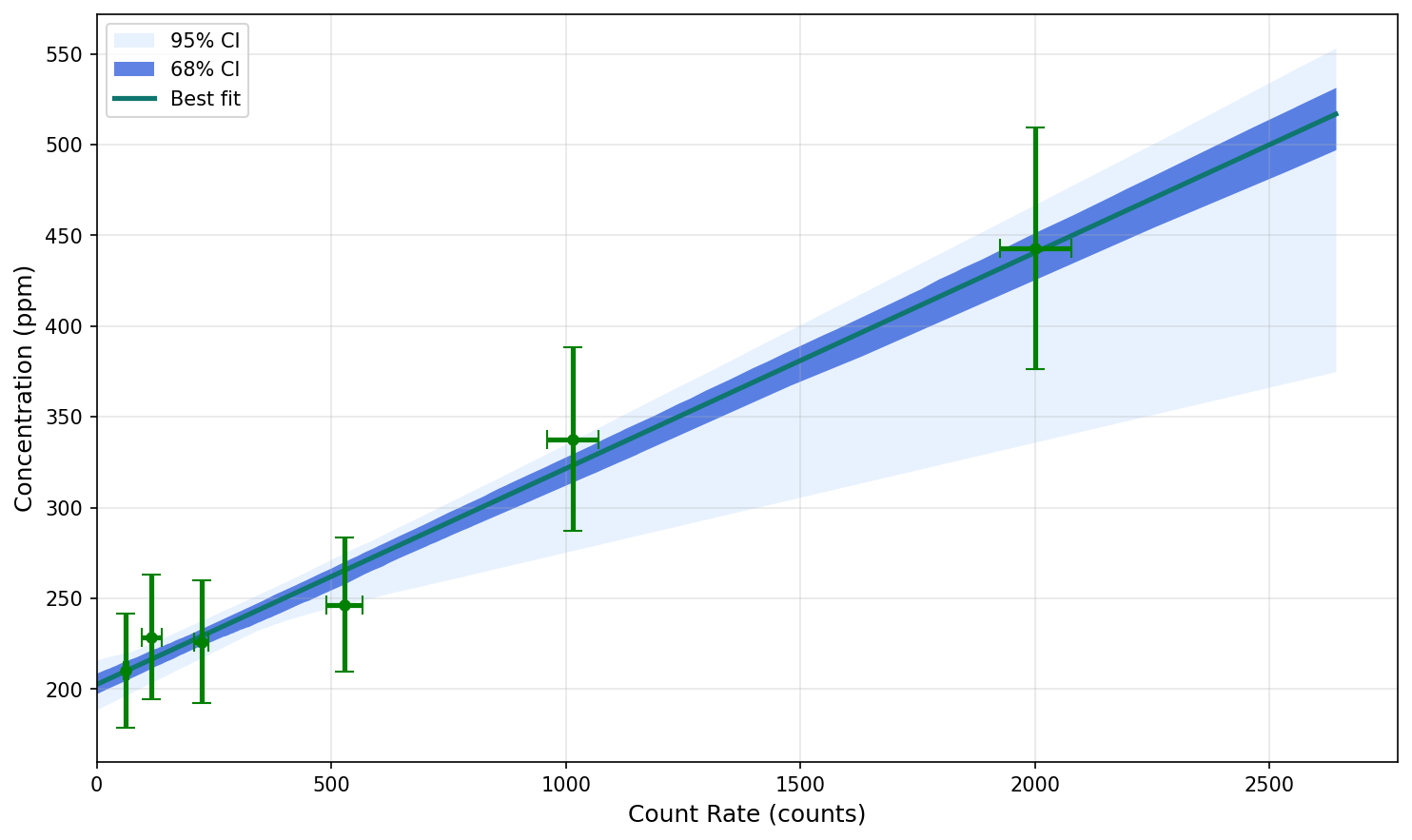
The shaded bands are the 68% (inner) and 95% (outer) bootstrap confidence intervals. Narrower bands indicate a more precisely constrained calibration.
Bootstrap parameter distributions
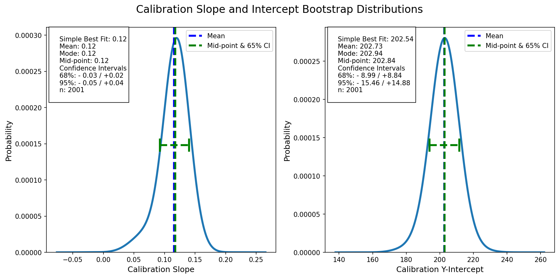
Each histogram shows how the fitted slope and intercept vary across bootstrap resamples, giving you a direct view of parameter uncertainty.
Fit with synthetic outliers
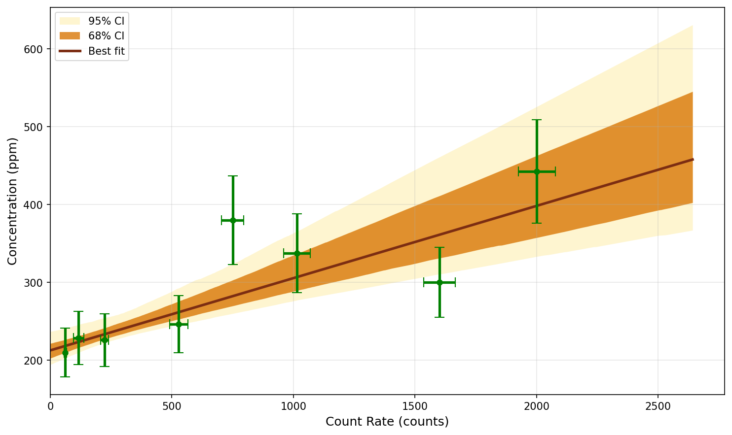
Including potential outliers in the regression widens the confidence bands and may shift the best-fit line. This illustrates why points that cannot be excluded objectively should be retained: the bootstrap distributions quantify their effect on the fitted parameters and prediction uncertainty.
Outlier-affected parameter distributions
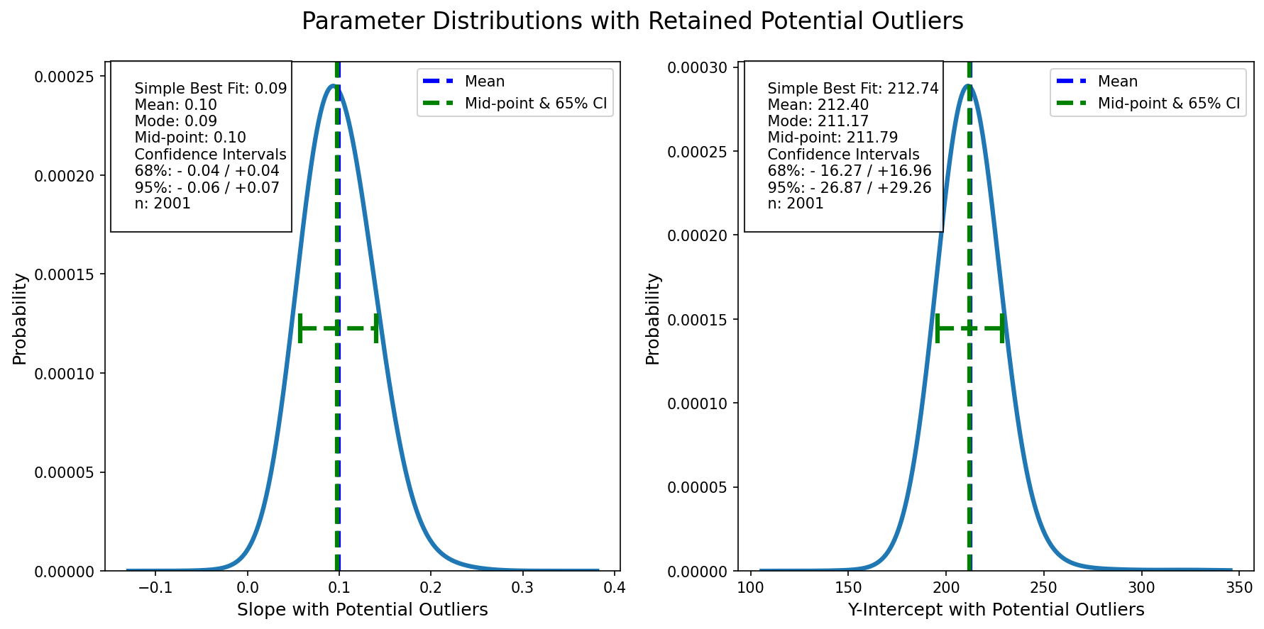
The potential outliers broaden and shift both distributions. Comparing these to the clean-data distributions makes their influence easy to quantify.
Module Functions
Defaults helper
fit_defaults(x, y, fit_intercept=True)
Computes sensible starting parameters from your data using a least-squares pre-fit.
Returns{"initial_guess": [...], "line_max": float, "line_interval": float}.
Core fitting
-
fit_odr_linear(x, y, x_err, y_err, fit_intercept=True, initial_guess=None)
Single ODR fit. Returns(params, param_errors). -
bootstrap_odr_fit(x, y, x_err, y_err, resample_draws, ...)
Fits the ODR model to N random resamples of your data.
Returns(all_fit_params, resampled_data).
Confidence intervals
-
evaluate_confidence(fit_params, line_max, line_interval, confidence_level=0.95)
Computes confidence bounds from bootstrap parameter distributions.
Returns a DataFrame indexed by x-values. -
odr_bootstrap(...)
Convenience wrapper: runsbootstrap_odr_fit+evaluate_confidencein one call.
line_max,line_interval, andinitial_guessare derived automatically when omitted.
Statistics
gaussian_aggregate(concentrations, errors)
Aggregates bootstrap distributions into a smooth KDE estimate.
Returns(distribution_dict, statistics_dict).
Plotting
-
plot_regression(confidence_df, datapoints=None, ax=None, ...)
Plots the best-fit line with shaded confidence band(s). -
plot_density(data, bounds, ax=None, ...)
Plots a probability density curve fromgaussian_aggregateoutput. -
plot_calibration_estimates(fit_params, fit_error, title=...)
Side-by-side slope and intercept distribution plots.
Requirements
- Python >= 3.11
- numpy >= 2.2.4
- scipy >= 1.15.2
- odrpack >= 0.6.1
- pandas >= 2.2.3
- matplotlib >= 3.10.1
License
MIT — see LICENSE.
Citation
@software{towbin2025odr,
  title  = {ODR Bootstrap: Orthogonal Distance Regression with Bootstrap Resampling},
  author = {Towbin, Henry},
  year   = {2025},
  url    = {https://github.com/whtowbin/odr_bootstrap_package}
}
1 maintainer

Metadata
1 maintainer
Release files for odr-bootstrap 2.1.0
For a detailed explanation of source distributions (sdists) and built distributions (wheels), please see the package formats documentation.
Source distribution (sdist)
| File | Size | Uploaded | |
|---|---|---|---|
| odr_bootstrap-2.1.0.tar.gz | 2.0 MB | Details |
Built distribution (wheel)
| File | Interpreter | ABI | Platform | Reset |
|---|---|---|---|---|
| odr_bootstrap-2.1.0-py3-none-any.whl | Python 3 | none | any | Details |
Total release size: 2.0 MB
Release files / odr_bootstrap-2.1.0.tar.gz
| Download URL | odr_bootstrap-2.1.0.tar.gz |
|---|---|
| Size | 2.0 MB |
| Tags | Source |
|
SHA-256 checksum How to use checksums |
2d2d82aaa16704ea8db804a470b664556cc8aad02471402ff898421cd3ce772b
|
|
BLAKE2b-256 checksum How to use checksums |
9034e446d0d0157e4974169ab4b019bf0da93e82b49cc63d7fe8e60b030bf8b6
|
| Upload date | |
|
Uploaded using Trusted Publishing? What is trusted publishing? |
No |
| Uploaded via |
uv/0.11.29 {"installer":{"name":"uv","version":"0.11.29","subcommand":["publish"]},"python":null,"implementation":{"name":null,"version":null},"distro":{"name":"macOS","version":null,"id":null,"libc":null},"system":{"name":null,"release":null},"cpu":null,"openssl_version":null,"setuptools_version":null,"rustc_version":null,"ci":null}
|
Release files / odr_bootstrap-2.1.0-py3-none-any.whl
| Download URL | odr_bootstrap-2.1.0-py3-none-any.whl |
|---|---|
| Size | 18.7 kB |
| Tags | Python 3 |
|
SHA-256 checksum How to use checksums |
b131998a89c739896a4316f6a1dc616b57152a66aa2a49c397896d1a0a62eee8
|
|
BLAKE2b-256 checksum How to use checksums |
630787317fc4c8d1775b9ce6c68cb078e876da07f193688034cfdeb905b310cd
|
| Upload date | |
|
Uploaded using Trusted Publishing? What is trusted publishing? |
No |
| Uploaded via |
uv/0.11.29 {"installer":{"name":"uv","version":"0.11.29","subcommand":["publish"]},"python":null,"implementation":{"name":null,"version":null},"distro":{"name":"macOS","version":null,"id":null,"libc":null},"system":{"name":null,"release":null},"cpu":null,"openssl_version":null,"setuptools_version":null,"rustc_version":null,"ci":null}
|














