Dual Octree Graph Neural Networks

Project description
Dual Octree Graph Networks


This repository contains a pure PyTorch-based implementation of our papers
Dual Octree Graph Networks (SIGGRAPH 2022). The code is released under the
MIT license. The experiments are conducted on Ubuntu 18.04 with 4 2080Ti
GPUs (12GB memory). The original implementation relies on C++ and CUDA and can be found
here, which has got


Dual Octree Graph Networks for Learning Adaptive Volumetric Shape Representations
Peng-Shuai Wang,
Yang Liu, and
Xin Tong
ACM Transactions on Graphics (SIGGRAPH), 41(4), 2022
- Dual Octree Graph Networks
1. Installation
-
Install PyTorch>=1.9.1 according to the official documentation of PyTorch. The code is tested with
PyTorch 1.12.1andcuda 11.3.Attention: Surprisingly, the code may be more than 5 times slower if the
PyTorchversion is2.x; the reseason might be that the scatter functions inPyTorch>2.xare much slower, which are key operations in our networks. -
Clone this repository and install other requirements.
git clone https://github.com/octree-nn/ognn-pytorch.git
cd  ognn-pytorch
pip install -r requirements.txt
2. Shape Reconstruction with ShapeNet
2.1 Data Preparation
-
Download
ShapeNetCore.v1.zip(31G) from ShapeNet and place it into the folderdata/ShapeNet. -
Convert the meshes in
ShapeNetCore.v1to signed distance fields (SDFs).python tools/shapenet.py --run convert_mesh_to_sdf
Note that this process is relatively slow, it may take several days to finish converting all the meshes from ShapeNet. And for simplicity, I did not use multiprocessing of Python to speed up. If the speed is a matter, you can simultaneously execute multiple Python commands manually by specifying the
startandendindex of the mesh to be processed. An example is shown as follows:python tools/shapenet.py --run convert_mesh_to_sdf --start 10000 --end 20000
The
ShapeNetConv.v1contains 57k meshes. After unzipping, the total size is about 100G. The total sizes of the generated SDFs and the repaired meshes are 450G and 90G, respectively. Please make sure your hard disk has enough space. -
Sample points and ground-truth SDFs for the learning process.
python tools/shapenet.py --run generate_dataset
-
If you just want to forward the pre-trained network, download the test point clouds (330M) manually from here and unzip them to the folder
data/ShapeNet/test.input, then download the filelists from here and unzip them to the folderdata/ShapeNet/filelist.
2.2 Experiment
-
Train: Run the following command to train the network on 4 GPUs. The training takes 21 hours on 4 2080Ti GPUs. The trained weight and log can be downloaded here.
python main.py --config configs/shapenet.yaml SOLVER.gpu 0,1,2,3
-
Test: Run the following command to generate the extracted meshes. It is also possible to specify other trained weights by replacing the parameter after
SOLVER.ckpt.python main.py --config configs/shapenet_eval.yaml \ SOLVER.ckpt logs/shapenet/shapenet/checkpoints/00300.model.pth
-
Evaluate: We use the code of ConvONet to compute the evaluation metrics. Following the instructions here to reproduce our results in Table 1.
2.3 Generalization
-
Test: Run the following command to test the trained network on unseen 5 categories of ShapeNet:
python main.py --config configs/shapenet_unseen5.yaml  \
       SOLVER.ckpt logs/shapenet/shapenet/checkpoints/00300.model.pth
-
Evaluate: Following the instructions here to reproduce our results on the unseen dataset in Table 1.
3. Synthetic Scene Reconstruction
3.1 Data Preparation
Download and unzip the synthetic scene dataset (205G in total) and the data splitting file lists by ConvONet via the following command. If needed, the ground truth meshes can be downloaded from here (90G).
python tools/room.py --run generate_dataset
3.2 Experiment
-
Train: Run the following command to train the network on 4 GPUs. The training takes about 41 hours on 4 2080Ti GPUs. The trained weight and log can be downloaded here.
python main.py --config configs/synthetic_room.yaml SOLVER.gpu 0,1,2,3
-
Test: Run the following command to generate the extracted meshes.
python main.py --config configs/synthetic_room_eval.yaml  \
    SOLVER.ckpt logs/room/room/checkpoints/00900.model.pth
-
Evaluate: Following the instructions here to reproduce our results in Table 5.
4. Unsupervised Surface Reconstruction with DFaust
4.1 Data Preparation
-
Download the DFaust dataset, unzip the raw scans into the folder
data/dfaust/scans, and unzip the ground-truth meshes into the folderdata/dfaust/mesh_gt. Note that the ground-truth meshes are used in computing evaluation metrics and NOT used in training. -
Run the following command to prepare the dataset.
python tools/dfaust.py --run genereate_dataset
-
For convenience, we also provide the dataset for downloading.
python tools/dfaust.py --run download_dataset
4.2 Experiment
-
Train: Run the following command to train the network on 4 GPUs. The training takes about 44 hours on 4 2080Ti GPUs. The trained weight and log can be downloaded here.
python main.py --config configs/dfaust.yaml SOLVER.gpu 0,1,2,3
-
Test: Run the following command to generate the meshes with the trained weights.
python main.py --config configs/dfaust_eval.yaml  \
       SOLVER.ckpt logs/dfaust/dfaust/checkpoints/00600.model.pth
-
Evaluate: To calculate the evaluation metric, we need first rescale the mesh into the original size, since the point clouds are scaled during the data processing stage.
python tools/dfaust.py  \
       --mesh_folder   logs/dfaust_eval/dfaust  \
       --output_folder logs/dfaust_eval/dfaust_rescale  \
       --run rescale_mesh
Then our results in Table 6 can be reproduced in the file
metrics.csv.python tools/compute_metrics.py \ --mesh_folder logs/dfaust_eval/dfaust_rescale \ --filelist data/dfaust/filelist/test.txt \ --ref_folder data/dfaust/mesh_gt \ --filename_out logs/dfaust_eval/dfaust_rescale/metrics.csv
4.3 Generalization
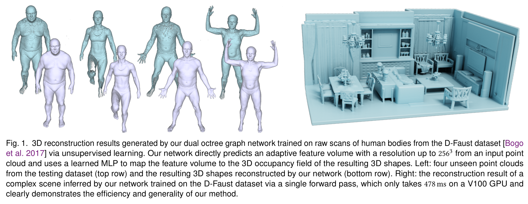
In Figure 1 and 11 of our paper, we test the generalization ability of our
network on several out-of-distribution point clouds. Please download the point
clouds from here,
and place the unzipped data to the folder data/shapes. Then run the following
command to reproduce the results:
python main.py --config configs/shapes.yaml  \
       SOLVER.ckpt logs/dfaust/dfaust/checkpoints/00600.model.pth
5. Autoencoder with ShapeNet
5.1 Data Preparation
Following the instructions here to prepare the dataset.
5.2 Experiment
-
Train: Run the following command to train the network on 4 GPUs. The training takes 25 hours on 4 2080Ti GPUs. The trained weight and log can be downloaded here.
python main.py --config configs/shapenet_ae.yaml SOLVER.gpu 0,1,2,3
-
Test: Run the following command to generate the extracted meshes.
python main.py --config configs/shapenet_ae_eval.yaml  \
       SOLVER.ckpt logs/shapenet/ae/checkpoints/00300.model.pth
-
Evaluate: Run the following command to evaluate the predicted meshes. Then our results in Table 7 can be reproduced in the file
metrics.4096.csv.python tools/compute_metrics.py \ --mesh_folder logs/shapenet_eval/ae \ --filelist data/ShapeNet/filelist/test_im.txt \ --ref_folder data/ShapeNet/mesh.test.im \ --num_samples 4096 \ --filename_out logs/shapenet_eval/ae/metrics.4096.csv
6. Citation
@article {Wang-SIG2022,
  title      = {Dual Octree Graph Networks
                for Learning Adaptive Volumetric Shape Representations},
  author     = {Wang, Peng-Shuai and Liu, Yang and Tong, Xin},
  journal    = {ACM Transactions on Graphics (SIGGRAPH)},
  volume     = {41},
  number     = {4},
  year       = {2022},
}


Download files
Download the file for your platform. If you're not sure which to choose, learn more about installing packages.
Source Distribution
Built Distribution
Filter files by name, interpreter, ABI, and platform.
If you're not sure about the file name format, learn more about wheel file names.
Copy a direct link to the current filters
File details
Details for the file ognn-1.1.2.tar.gz.
File metadata
- Download URL: ognn-1.1.2.tar.gz
- Upload date:
- Size: 27.3 kB
- Tags: Source
- Uploaded using Trusted Publishing? No
- Uploaded via: twine/6.0.1 CPython/3.9.19
File hashes
| Algorithm | Hash digest | |
|---|---|---|
| SHA256 |
b4f002a534876c07d9518efd211549a2cc2bba1a2e6d97db574fa7d0bb19d3fa
|
|
| MD5 |
1ca1e88fc7f517220b803ac869ba0ffd
|
|
| BLAKE2b-256 |
969280515afd94a9312b03ecd931e1274046c5e7cb2f7acffdc19b3d1536d39a
|
File details
Details for the file ognn-1.1.2-py3-none-any.whl.
File metadata
- Download URL: ognn-1.1.2-py3-none-any.whl
- Upload date:
- Size: 32.3 kB
- Tags: Python 3
- Uploaded using Trusted Publishing? No
- Uploaded via: twine/6.0.1 CPython/3.9.19
File hashes
| Algorithm | Hash digest | |
|---|---|---|
| SHA256 |
def2265970df19d17e5cf2e435e5dd7d51d49a2432cbcc234fddc660d3bb06ed
|
|
| MD5 |
bdb39cb1ffc86e8e42b0f25ac3562d23
|
|
| BLAKE2b-256 |
4e409c0a8becf92d0abcca041703db2acc121caffa709d2f3ebe92336759d632
|


