Generate probability distributions on the future price of publicly traded securities using options data

Project description


Overview
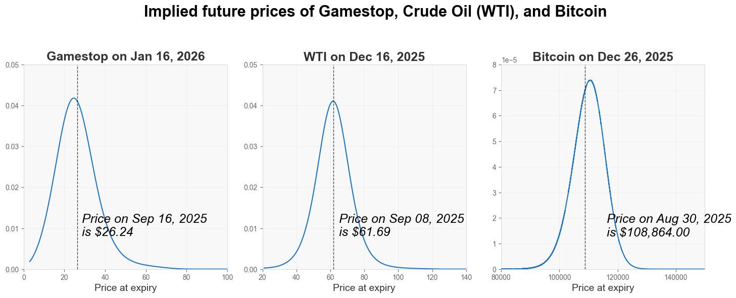
OIPD computes the probabilities implied by the options market for an asset’s future prices.
It does this by taking listed options data, fitting an arbitrage-free implied volatility curve or surface, and then transforming that fitted object into a probability distribution over future asset prices. In practice, that provides two core capabilities in one library:
- Volatility modeling: fit single-expiry smiles and multi-expiry volatility surfaces for pricing and risk work.
- Probability extraction: compute market-implied probability distributions, cumulative probabilities, quantiles, and distributional moments.

|

|
See the full documentation site for details.
Quick start
1. Installation
pip install oipd
2. Mental model for using OIPD
[!TIP] For non-technical users, you can safely skip this section and jump to Section 3 to compute future market-implied probabilities.
OIPD has four core objects.
A simple way to understand the package is by use case: fitting at a single future date vs over time, and working in implied volatility vs probabilities.
| Scope | Volatility Layer | Probability Layer |
|---|---|---|
| Single future date | VolCurve |
ProbCurve |
| Future time horizon | VolSurface |
ProbSurface |
You can think about the lifecycle in three steps:
- Initialize the estimator object with configuration.
- Call
.fit(chain, market)to calibrate. - Query/plot the fitted object, or convert from vol to probability via
.implied_distribution().
If you're familiar with scikit-learn, this is the same mental model: configure an estimator, call fit, then inspect outputs.
Conceptual flow:
Step 1: Fit volatility
  Initialize VolCurve / VolSurface object
      + options chain + market inputs
      -> .fit(...)
      -> fitted VolCurve / VolSurface object (inspect IV, prices, greeks, etc.)

Step 2: Convert fitted volatility to probability
  Use fitted VolCurve / VolSurface
      -> .implied_distribution()
      -> ProbCurve / ProbSurface object (inspect PDF, CDF, quantiles, moments, etc.)
3. Quickstart tutorial in computing market-implied probability distributions
This quickstart will cover the functionality in (1) computing market-implied probabilities. See the included jupyter notebook for a full example on using the automated yfinance connection to download options data and compute market-implied probabilities for Palantir.
For a more technical tutorial including the functionality of (2) volatility fitting, see the additional jupyter notebooks in the examples directory, as well as the full documentation.
3A. Usage for computing a probability distribution on a specific future date
import matplotlib.pyplot as plt

from oipd import MarketInputs, ProbCurve, sources

# 1. we download data using the built-in yfinance connection
ticker = "PLTR"                               # specify the stock ticker
expiries = sources.list_expiry_dates(ticker)  # see all expiry dates
single_expiry = expiries[1]                   # select one of the expiry dates you're interested in

chain, snapshot = sources.fetch_chain(ticker, expiries=single_expiry) # download the options chain data, and a snapshot at the time of download

# 2. fill in the parameters
market = MarketInputs(
    valuation_date=snapshot.asof,               # datetime on which the options data was downloaded
    underlying_price=snapshot.underlying_price, # the price of the underlying stock at the time when the options data was downloaded
    risk_free_rate=0.04,                        # the risk-free rate of return. Use the US Fed or Treasury yields that are closest to the horizon of the expiry date
)

# 3. compute the future probability distribution using the data and parameters
prob = ProbCurve.from_chain(chain, market)

# 4. query the computed result to understand market-implied probabilities and other statistics
prob.plot()
plt.show()

prob_below = prob.prob_below(100)   # P(price < 100)
prob_above = prob.prob_above(120)   # P(price >= 120)
q50 = prob.quantile(0.50)           # median implied price
skew = prob.skew()                  # skew

3B. Usage for computing probabilities over time
import matplotlib.pyplot as plt

from oipd import MarketInputs, ProbSurface, sources

# 1. download multi-expiry data using the built-in yfinance connection
ticker = "PLTR"
chain_surface, snapshot_surface = sources.fetch_chain(
    ticker,
    horizon="12m",  # auto-fetch all listed expiries inside the horizon
)

# 2. fill in the parameters
surface_market = MarketInputs(
    valuation_date=snapshot_surface.asof,               # datetime on which the options data was downloaded
    underlying_price=snapshot_surface.underlying_price, # price of the underlying stock at download time
    risk_free_rate=0.04,                                # risk-free rate for the horizon
)

# 3. compute the probability surface using the data and parameters
surface = ProbSurface.from_chain(chain_surface, surface_market)

# 4. query and visualize the surface
surface.plot_fan() # Plot a fan chart of price probability over time
plt.show()

# 5. query at arbitrary maturities directly from ProbSurface
pdf_45d = surface.pdf(100, t=45/365)                      # density at K=100, 45.0 ACT/365 days from valuation_date
cdf_intraday = surface.cdf(100, t="2025-02-15 09:30:00")  # example timestamp-style maturity input
q50_45d = surface.quantile(0.50, t=45/365)                # median at 45 days

# 6. "slice" the surface to get a ProbCurve, and query its statistical properties in the same manner as in example A
surface.expiries                                  # list all the expiry dates that were captured
curve = surface.slice(surface.expiries[0]) # get a slice on the first expiry
curve.prob_below(100)                      # query probabilities and statistics
curve.kurtosis()

OIPD also supports manual CSV or DataFrame uploads.
See more examples for demos.
Community
Pull requests welcome! Reach out on GitHub issues to discuss design choices.
Join the Discord community to share ideas, discuss strategies, and get support. Message me with your feature requests, and let me know how you use this.
Contributors
Thanks to everyone who has contributed code:

And special thanks for support on theory, implementation, or advisory:
- integral-alpha.com
- Jannic H., Chun H. H., and Melanie C.
- and others who prefer to go unnamed
Release history Release notifications | RSS feed


Download files
Download the file for your platform. If you're not sure which to choose, learn more about installing packages.
Source Distribution
Built Distribution
Filter files by name, interpreter, ABI, and platform.
If you're not sure about the file name format, learn more about wheel file names.
Copy a direct link to the current filters
File details
Details for the file oipd-2.0.3.tar.gz.
File metadata
- Download URL: oipd-2.0.3.tar.gz
- Upload date:
- Size: 218.3 kB
- Tags: Source
- Uploaded using Trusted Publishing? No
- Uploaded via: twine/6.2.0 CPython/3.12.6
File hashes
| Algorithm | Hash digest | |
|---|---|---|
| SHA256 |
c8c43319d5d05764ec59a5f67cd569beedbb806eb122c565cf2bfaf771115673
|
|
| MD5 |
648fdd5a65992c0bb436e2ce8e3529cc
|
|
| BLAKE2b-256 |
93612716c8e38bc62f52ec6d4acf2d5fb61262b5ec92596ebdf6d789c0591195
|
File details
Details for the file oipd-2.0.3-py3-none-any.whl.
File metadata
- Download URL: oipd-2.0.3-py3-none-any.whl
- Upload date:
- Size: 203.5 kB
- Tags: Python 3
- Uploaded using Trusted Publishing? No
- Uploaded via: twine/6.2.0 CPython/3.12.6
File hashes
| Algorithm | Hash digest | |
|---|---|---|
| SHA256 |
0a06a02fd488837b092ed07389cf46a93f59debcab5f7114130c39327ba0965c
|
|
| MD5 |
22346efa051782aa3ef43aeefb49057a
|
|
| BLAKE2b-256 |
c6cba7e0cd6e8d174112bef7ad12649b81be66a687f16c8015c45b384f95dd11
|


