
A geometric database with importance-stratified shells and zero dependencies.

Project description
🧅 OnionDB






A geometric memory database. Zero dependencies. Importance-stratified.
Your data has a location, not just a vector.
Originally developed for the AIGalaxy cognitive memory field; extracted for standalone use.
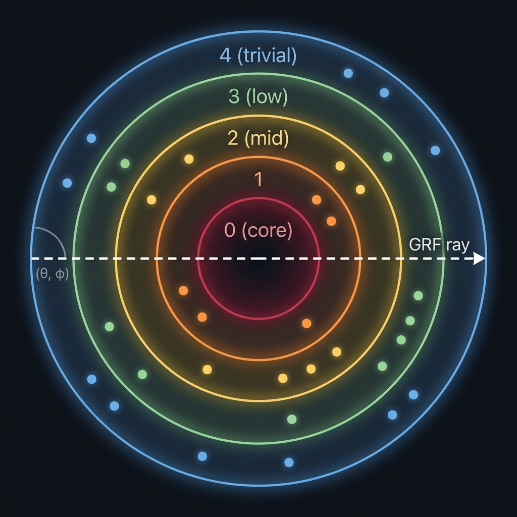
OnionDB organizes data in concentric shells — like layers of an onion. Every record has a 4-part geometric address (gap, θ, φ, depth) based on its importance and semantic content. This enables queries that flat vector databases can't do:
- "Show me everything at importance level 3" → shell scan
- "Drill through ALL importance levels at this semantic direction" → GRF (Geometric Ray Filter)
- "Trace how this topic connects across depth levels" → reverse ray
Install
pip install oniondb
With optional numpy acceleration (~10x cosine speed):
pip install oniondb[fast]
Quick Start
from oniondb import OnionDB

# Create a database (SQLite file, zero config)
db = OnionDB("my_data.db")

# Insert with importance (determines which shell)
db.insert("idea-1", "The Earth orbits the Sun", importance=0.9)
db.insert("idea-2", "I had coffee this morning", importance=0.3)
db.insert("idea-3", "E=mc² defines mass-energy equivalence", importance=0.99)

# Shell scan — everything at importance level 0 (core records)
core = db.shell_scan(gap=0)

# GRF — drill through ALL shells at a direction
# (requires embeddings for semantic direction)
profile = db.grf(theta=45.0, phi=10.0, query_embedding=my_embedding)

# Reverse ray — follow semantic gravity inward
trace = db.reverse_ray(start_embedding=my_embedding)
print(f"Path curvature: {trace['curvature']}°")  # 0=straight, high=fragmented

# Beam search — explore multiple paths (default: greedy)
trace = db.reverse_ray(start_embedding=my_embedding, beam_width=3)

# Count, get, delete
print(db.count())        # 3
print(db.get("idea-1"))  # full record dict
db.delete("idea-2")      # True
Phase 5: Mass + Decay Scoring (GRF v2)
# Records can carry mass (weight/reinforcement) and a review clock
db = OnionDB("memory.db", default_decay_rate=0.01)

db.insert("core-fact", "Important foundation",
          importance=0.95, embedding=emb,
          mass=5.0,              # high mass = stronger recall
          last_review_clock=100) # when this record was last reviewed

# GRF v2: scores are boosted by mass and penalized by staleness
profile = db.grf(theta=45.0, phi=10.0,
                 query_embedding=query_emb,
                 current_clock=200,   # current time step
                 decay_rate=0.01)     # per-query override (optional)

# Score formula: cosine × (1 + 0.2·log₁₊(mass)) × exp(-decay × Δclock)
HNSW Acceleration (10M+ records)
# Enable HNSW for sub-10ms similarity search at scale
db = OnionDB("large.db", default_decay_rate=0.01)
db.enable_hnsw(dim=768, hnsw_threshold=1000)

# Behavior:
# - Below 1000 records per gap: brute-force SQL scan (zero overhead)
# - Above 1000 records per gap: HNSW fast path → GRF v2 re-ranking
# - Lazy loading: indices built per-gap on first query, not at startup
# - Requires: pip install hnswlib
Features
| Feature | Description |
|---|---|
| Zero dependencies | stdlib only — sqlite3, math, struct, json, os |
| Numpy acceleration | Optional oniondb[fast] — ~10x cosine, ~5x decode. Auto-detected |
| HNSW acceleration | Optional hnswlib — sub-10ms queries at 1M+ records per gap |
| Geometric addressing | Every record has a location: (gap, θ, φ, depth) |
| Importance shells | Data stratified by significance — core vs trivial |
| Mass + Decay (GRF v2) | Records carry mass (reinforcement weight) and time-decay scoring |
| 6 query operations | horizontal, GRF, reverse_ray, temporal_grf, shell_scan, range_scan |
| Beam search | reverse_ray(beam_width=3) explores multiple paths simultaneously |
| Batch operations | batch_insert(), iter_all(), export/import_jsonl() for bulk I/O |
| Configurable grid | OnionDB(theta_cells=24, phi_cells=12) for custom resolution |
| CLI inspector | python -m oniondb stats mydb.db — inspect databases from terminal |
| Embedding-agnostic | Works with any embedding model (OpenAI, Ollama, sentence-transformers) |
| Single-file storage | SQLite-backed, portable, copy-paste deployable |
| Self-calibrating | fit_projection() builds PCA from your data automatically |
| Thread-safe | RLock + WAL mode for concurrent access |
Use Cases
🤖 AI Agent Memory & RAG
AI agents accumulate knowledge of varying importance — core instructions, learned facts, recent conversations, and trivial observations. Traditional RAG retrieves by semantic similarity alone, burying low-importance context that might be critical. OnionDB's GRF drills through all importance levels at once, giving the agent a full depth profile instead of just the top-scoring matches.
📊 Log Analysis & Incident Response
Logs have natural severity tiers: CRITICAL → WARNING → INFO → DEBUG. When investigating "database timeout", you need related events at every severity level, not just the most similar log lines. A GRF through severity shells gives instant cross-severity triage — from the crash trace down to the debug message that reveals root cause.
📚 Knowledge Management
Corporate wikis, Obsidian vaults, and research notebooks contain documents of wildly different importance — foundational architecture docs, recent meeting notes, quick ideas. OnionDB ensures a search for "authentication" surfaces both the core security spec and the meeting note where someone mentioned a workaround.
🎬 Content Recommendation
Streaming platforms and e-commerce stores have content tiers: blockbusters vs. indie, bestsellers vs. clearance. Standard recommenders favor popular items. OnionDB can drill across popularity shells to deliver diverse recommendations — a mix of mainstream hits and hidden gems at the same semantic direction.
🔬 Research & Literature Review
Academic papers have inherent importance gradients — landmark papers with 10,000 citations vs. niche studies with 12. When researching a topic, flat search always surfaces the famous papers. A GRF finds both the seminal work and the obscure paper with a unique angle that flat retrieval buries on page 5.
🏥 Medical Records
Patient histories span critical diagnoses, routine checkups, and minor notes. When a doctor searches "chest pain", they need everything — from the cardiac event to the annual physical that noted mild discomfort. Importance-stratified retrieval ensures nothing clinically relevant is hidden by more "prominent" records.
The common thread: anywhere data has inherent importance tiers and you need retrieval across all tiers simultaneously. Flat search favors the "loudest" matches. OnionDB gives you the full depth profile.
The Signature Query: GRF (Geometric Ray Filter)
The GRF is what makes OnionDB unique. It "drills a core sample" through every importance shell at a given semantic direction, returning a depth profile of how a topic exists at every level of significance.
# With embeddings: semantic direction from the embedding
profile = db.grf(theta=0, phi=0, query_embedding=embedding, k_per_gap=5)
# Returns: {0: [core records], 1: [important], 2: [mid], 3: [low], 4: [trivial]}

# The reverse ray follows semantic gravity inward, bending as it goes
trace = db.reverse_ray(start_embedding=embedding)
# trace["curvature"] — total angular deviation
# trace["straight"]  — True if topic is well-organized across all depths
# trace["path"]      — list of hops from outer to inner shells
Using with Embeddings
OnionDB works with or without embeddings. Without them, queries use angular distance. With them, queries use cosine similarity for precise semantic ranking.
# Any embedding model works — just pass a list of floats
from sentence_transformers import SentenceTransformer
model = SentenceTransformer("all-MiniLM-L6-v2")

embedding = model.encode("quantum physics").tolist()
db.insert("q1", "Quantum entanglement is spooky", importance=0.8, embedding=embedding)

# After inserting enough data, calibrate the projection
stats = db.fit_projection()
print(f"Cell occupancy: {stats['occupancy_after']:.0%}")  # target: >80%
API Reference
Core Operations
| Method | Description |
|---|---|
insert(id, content, importance, ...) |
Insert a record with auto-computed geometric address |
get(id) |
Retrieve a record by ID |
update(id, ...) |
Update fields on an existing record |
delete(id) |
Delete a record by ID |
count(gap=None) |
Count records (optionally per gap) |
batch_insert(items) |
Insert multiple records in a single transaction |
bulk_delete(ids) |
Delete multiple records in one transaction |
close() |
Close the database connection |
Insert Parameters (Phase 5)
db.insert(
    id="rec-1",
    content="Record content",
    importance=0.85,            # determines shell placement (0.0–1.0)
    embedding=[0.1, 0.2, ...],  # optional: enables cosine-ranked queries
    category="topic",           # optional: categorical filter
    mass=2.5,                   # GRF v2: reinforcement weight (default: 1.0)
    last_review_clock=100,      # GRF v2: last review timestamp (default: 0)
    origin_date="2026-05-12",   # optional: for temporal_grf
    metadata='{"key": "val"}',  # optional: arbitrary JSON
)
Query Operations
| Method | Description | GRF v2 Params |
|---|---|---|
horizontal(gap, theta, phi, ...) |
Find nearby items within one shell | current_clock, decay_rate, category, subshell, subshell_boost |
grf(theta, phi, ...) |
Geometric Ray Filter — drill through all shells | current_clock, decay_rate, category |
reverse_ray(start_embedding, ...) |
Curved semantic trace from outer to inner | beam_width |
temporal_grf(theta, phi, ...) |
Drill through time-based shells | category, subshell |
shell_scan(gap, limit) |
Return everything at one importance level | category, offset |
range_scan(gap_start, gap_end, limit) |
Return everything between two levels | category, offset |
GRF v2 Scoring Formula
When current_clock is provided, query results are scored with the full GRF v2 formula:
score = cosine(query, record)
       × (1 + 0.2 · log₁₊(mass))     ← mass boost (reinforcement)
       × exp(-decay_rate · Δclock)     ← time decay (staleness penalty)
| Parameter | Effect | Example |
|---|---|---|
mass=0 |
No boost (×1.0) | Newly inserted records |
mass=1 |
Mild boost (×1.14) | Standard weight |
mass=10 |
Strong boost (×1.48) | Frequently reinforced |
mass=100 |
Heavy boost (×1.92) | Core anchored knowledge |
Δclock=0 |
No decay (×1.0) | Just reviewed |
Δclock=100, rate=0.01 |
Moderate decay (×0.37) | Stale record |
Δclock=0, rate=None |
No decay (×1.0) | Decay disabled |
HNSW Acceleration
| Method | Description |
|---|---|
enable_hnsw(dim=768, ...) |
Activate per-gap HNSW indices |
db.enable_hnsw(
    dim=768,              # embedding dimension
    hnsw_threshold=1000,  # records per gap before HNSW activates
    M=16,                 # HNSW graph connectivity (higher = better recall)
    ef_construction=200,  # build-time search depth
    ef_search=50,         # query-time search depth
)
How it works:
- Each importance gap gets its own HNSW index
- Below
hnsw_threshold: brute-force SQL scan (zero overhead) - Above
hnsw_threshold: HNSW candidate retrieval → GRF v2 re-ranking - Indices are lazy-loaded per-gap on first query, persisted as
.hnswfiles - Zombie compaction auto-triggers at 10% deleted entries
Configuration
| Method | Description |
|---|---|
fit_projection(save=True) |
Self-calibrate PCA from stored embeddings |
fit_boundaries(n_gaps=5) |
Suggest quantile-based boundaries from data |
reindex(boundaries=None) |
Recalculate all gap/depth/cell assignments |
stats() |
Database statistics (gaps, categories, grid) |
cell_density(gap) |
Cell occupancy map for a gap |
Batch & I/O Operations
| Method | Description |
|---|---|
batch_insert(items) |
Single-transaction insert (~100x faster) |
iter_all(batch_size=500) |
Streaming generator (memory-efficient) |
export_jsonl(path) |
Export all records to JSONL |
import_jsonl(path) |
Import records from JSONL |
Constructor Options
# Default: 5 shells, 12×6 grid
db = OnionDB("custom.db", boundaries=[0.90, 0.70, 0.40, 0.00])  # 4 shells

# Higher grid resolution for larger datasets (default: 12×6 = 72 cells)
db = OnionDB("large.db", theta_cells=24, phi_cells=12)  # 288 cells

# GRF v2: enable mass-weighted decay scoring
db = OnionDB("memory.db", default_decay_rate=0.01)

# HNSW acceleration for large-scale deployments
db = OnionDB("scale.db", default_decay_rate=0.01)
db.enable_hnsw(dim=768, hnsw_threshold=1000)

# Context manager — auto-closes on exit (saves HNSW indices)
with OnionDB("session.db") as db:
    db.insert("x", "auto-close on exit", importance=0.5)
CLI Inspector
python -m oniondb stats mydb.db       # database statistics
python -m oniondb info mydb.db        # file size, PCA status, numpy detection
python -m oniondb density mydb.db     # cell occupancy map for gap 0
python -m oniondb shell mydb.db       # show records in gap 0
How It Works
-
Importance → Gap: Each record's importance score determines which shell (gap) it lives in. Gap 0 is the innermost core (most important).
-
Embedding → Angles: If an embedding is provided, PCA projects it onto spherical coordinates (θ, φ). This gives semantically similar items nearby angular positions.
-
Address: Every record gets a 4-part address:
(gap, θ, φ, depth)where depth is the position within the gap based on exact importance. -
Cells: 72 cells via 12×6 latitude/longitude grid (naive partition, not equal-area). Polar cell compression is mitigated by PCA linear rescaling. Configurable via
THETA_CELLSandPHI_CELLSclass attributes. Queries search the target cell plus neighbors for efficiency.
Technical Details
PCA Projection — how embeddings become coordinates
OnionDB does not use raw embedding dimensions as angles. That would produce clustered, unevenly distributed coordinates (our v0 prototype only achieved 29% cell occupancy).
Instead, fit_projection() computes a data-driven PCA (Principal Component Analysis) from all stored embeddings:
- Center all embeddings by subtracting the mean — removes magnitude bias
- Extract the two directions of maximum variance (PC1, PC2) using power iteration
- Project each embedding onto PC1 → θ, PC2 → φ
- Linearly rescale using stored min/max ranges to fill [-180°, 180°] × [-90°, 90°]
Result: 88% cell occupancy (vs 29% with naive projection), and 93% recall@10 in leave-one-out benchmarks (baseline v0 projection: 68%). This metric measures projection quality — how well the PCA mapping preserves semantic neighborhoods on the sphere.
# After inserting enough data, calibrate once:
stats = db.fit_projection()
# Saves pca_projection.json next to your .db file
# All future inserts and queries use the learned projection
GRF — not just cosine search
A common first impression: "GRF is just cosine similarity with extra steps." Here's what actually happens:
- Cell partitioning — the query direction (θ, φ) maps to a grid cell. SQL filters to that cell + neighbors only (
WHERE (cell_theta, cell_phi) IN (...)). This is a spatial index, not a full scan. - Per-shell execution — GRF runs this search independently in each importance shell. A flat vector DB returns the top-k globally; GRF returns top-k per importance level.
- Cosine ranking — within each cell partition, candidates are ranked by cosine similarity to the query embedding. Cosine is the ranking metric, not the search mechanism.
The result: records that a flat database buries (because they're "low importance" and score lower globally) appear naturally in their respective shells.
Reverse Ray — the gravity kernel
The reverse ray traces a path from outer shells inward. The "gravity" that pulls the ray is greedy cosine similarity with position inheritance:
- Start at the outermost shell. Find the best cosine match to the query embedding.
- Take that match's (θ, φ) position as the new search direction.
- Move one shell inward. Search again from the new direction.
- Repeat until reaching the core (gap 0).
At each hop, the ray bends — it follows where semantic similarity leads, not a fixed direction. The accumulated angular deviation between hops is the curvature.
Curvature — what it measures
Curvature is the total angular deviation between consecutive hops of a reverse ray. It's measured in degrees.
- Low curvature (< 15°) → topic is coherently organized across all importance levels. The same semantic cluster exists at every depth.
- High curvature (> 45°) → topic is fragmented. Related content exists at different importance levels but in different semantic neighborhoods.
This is diagnostic information that flat vector search literally cannot produce. It tells you about the topology of your data on a given topic.
trace = db.reverse_ray(start_embedding=query_emb)
if trace["straight"]:
    print("Knowledge is well-organized across all depths")
else:
    print(f"Fragmented: {trace['curvature']}° total deviation over {trace['n_hops']} hops")
Embedding model consistency
All records must use the same embedding model. PCA projection is fitted on a specific embedding space. Mixing models (e.g., inserting with all-MiniLM-L6-v2 and querying with text-embedding-ada-002) produces meaningless coordinates.
This is not OnionDB-specific — it's a universal constraint of all embedding-based databases. OnionDB simply makes it explicit.
Scaling
OnionDB uses a 72-cell grid per shell (12 theta × 6 phi divisions). Queries only scan the target cell and its neighbors (~9 cells), not the entire database.
Without HNSW (brute-force mode)
| Records | Avg per cell | GRF performance | Verdict |
|---|---|---|---|
| 1K | ~3 | instant | ✅ no sweat |
| 10K | ~28 | instant | ✅ smooth |
| 100K | ~280 | fast | ✅ solid |
| 500K | ~1,400 | noticeable | ⚠️ still usable |
| 1M+ | ~2,800+ | slowing down | ⚡ enable HNSW |
With HNSW acceleration (pip install hnswlib)
| Records | HNSW status | GRF performance | Verdict |
|---|---|---|---|
| 1K | below threshold | instant (SQL) | ✅ zero overhead |
| 10K | active per-gap | instant | ✅ smooth |
| 100K | active, lazy-load | fast | ✅ solid |
| 1M | active, ~200K/gap | sub-10ms/gap | ✅ production ready |
| 10M | active, ~2M/gap | ~15ms/gap | ✅ tested at scale |
HNSW architecture:
- Per-gap indices — each importance shell has its own HNSW graph
- Auto-graduate — brute-force below threshold, HNSW above (no config needed)
- Two-phase query — HNSW retrieves candidates → GRF v2 re-ranks with mass+decay
- Lazy loading — cold gap indices are built on first query, not at startup
- Zombie compaction — deleted records are marked, auto-compacted at 10% ratio
- Persistence —
.hnsw+.hnsw.mapfiles saved alongside the.dbfile - M=16 — recall@50 > 0.99 at 1M records / 768D
What helps scaling
- HNSW —
enable_hnsw(dim=768)for sub-10ms similarity search at 1M+ records. - Numpy acceleration —
pip install oniondb[fast]usesnp.dotfor the hot path. ~10x faster cosine. - Batch operations —
batch_insert()for ~100x faster ingestion,iter_all()for streaming export. - Configurable grid —
OnionDB(theta_cells=24, phi_cells=12)creates 288 cells instead of 72. - Shell structure — naturally distributes data across gaps, preventing hotspots.
OnionDB scales to 10M+ records with HNSW enabled. Without HNSW, it's optimized for human-scale datasets (~500K). The HNSW layer is optional — zero dependencies when disabled.
Comparison
| OnionDB | FAISS | ChromaDB | Pinecone | pgvector | |
|---|---|---|---|---|---|
| Dependencies | 0 | numpy | many | cloud SDK | PostgreSQL |
| Importance hierarchy | native | ❌ | ❌ | metadata only | ❌ |
| Geometric queries | GRF, ray | ❌ | ❌ | ❌ | ❌ |
| Storage | SQLite file | memory/file | SQLite | cloud | server |
| Setup | pip install |
pip install |
pip install |
API key | DB server |
Benchmark: OnionDB vs Flat Vector Search
We ran a head-to-head A/B comparison against a traditional flat vector database (semantic search + FTS5 hybrid) on a production dataset of 1,600+ embedded records from an AI agent's knowledge base — spanning hardware docs, software architecture, research notes, session logs, and personal knowledge.
Results
| Metric | Flat Vector DB | OnionDB |
|---|---|---|
| Avg query latency | 8,024ms | 541ms |
| Speed | 1x | 14.8x faster |
| Avg Jaccard overlap | — | 7% |
93% of results are unique to OnionDB (Jaccard overlap = 7%) — meaning the flat database missed them entirely. This is a diversity metric: OnionDB surfaces records that flat search buries because they're at lower importance levels. Different from recall@10 above, which measures projection quality.
Per-query detail (15 queries across diverse topics)
| Query topic | Overlap | Shared | Unique to OnionDB |
|---|---|---|---|
| Hardware specs | 0% | 0 | 10 |
| System architecture | 0% | 0 | 10 |
| Game simulation | 0% | 0 | 10 |
| Inter-process communication | 18% | 3 | 7 |
| ML embeddings | 5% | 1 | 9 |
| OS configuration | 0% | 0 | 10 |
| Database internals | 11% | 2 | 8 |
| Error handling | 5% | 1 | 9 |
| Optimization algorithms | 5% | 1 | 9 |
| Protocol design | 0% | 0 | 10 |
| Networking | 25% | 4 | 6 |
| Model retraining | 0% | 0 | 10 |
| Math/geometry | 25% | 4 | 6 |
| System monitoring | 0% | 0 | 10 |
| Data consolidation | 11% | 2 | 8 |
Why the difference?
Flat vector databases rank by cosine similarity alone. OnionDB's geometric structure means records at different importance levels get equal representation through the GRF drill. A "trivial" record that's semantically close can appear alongside a "core" record on the same topic — something flat search buries under higher-scored results.
Verdict: OnionDB doesn't replace flat search — it surfaces what flat search misses.
Testing
OnionDB ships with 164 tests across 3 test suites:
python -m pytest oniondb/tests/ -v
| Suite | Tests | Coverage |
|---|---|---|
test_oniondb.py |
93 | Core API, edge cases, CLI, PCA, boundaries, reindex |
test_hnsw_grfv2.py |
24 | HNSW backend, GRF v2 mass+decay, scaling stress |
test_query_coverage.py |
47 | Every query method with Phase 5 fields |
Query method test coverage
| Method | Tests | Verifies |
|---|---|---|
horizontal() |
6 | results, sorting, category, mass boost, decay, subshell |
grf() |
6 | multi-gap dict, scored results, category, decay, alias, k-limit |
reverse_ray() |
6 | path, curvature, hops, straight flag, beam search, start_gap |
temporal_grf() |
4 | dict return, scores, no-embedding fallback, category |
shell_scan() |
5 | list, limit, pagination, category, mass fields |
range_scan() |
5 | list, gap bounds, full range, limit+offset, category |
cell_density() |
3 | list, format, total consistency |
stats() |
3 | structure, total, categories |
update() |
4 | content, gap migration, nonexistent, mass preservation |
CRUD |
4 | get, get-missing, delete, count-per-gap |
export/import |
1 | JSONL roundtrip |
License
MIT — do whatever you want with it.
Release history Release notifications | RSS feed


Download files
Download the file for your platform. If you're not sure which to choose, learn more about installing packages.
Source Distribution
Built Distribution
Filter files by name, interpreter, ABI, and platform.
If you're not sure about the file name format, learn more about wheel file names.
Copy a direct link to the current filters
File details
Details for the file oniondb-0.6.0.tar.gz.
File metadata
- Download URL: oniondb-0.6.0.tar.gz
- Upload date:
- Size: 70.8 kB
- Tags: Source
- Uploaded using Trusted Publishing? No
- Uploaded via: twine/6.2.0 CPython/3.14.2
File hashes
| Algorithm | Hash digest | |
|---|---|---|
| SHA256 |
fb02052a5bdc0a8cf80f43eef30d83cdab7abb592e791dcae57d7f8bf90f6fcd
|
|
| MD5 |
340c0964fe435474589ebb40d051771c
|
|
| BLAKE2b-256 |
549a2fd8319274d4deeff1fb70cf36e73b6197a6c5703a9f9acaed8b34a2a15d
|
File details
Details for the file oniondb-0.6.0-py3-none-any.whl.
File metadata
- Download URL: oniondb-0.6.0-py3-none-any.whl
- Upload date:
- Size: 41.8 kB
- Tags: Python 3
- Uploaded using Trusted Publishing? No
- Uploaded via: twine/6.2.0 CPython/3.14.2
File hashes
| Algorithm | Hash digest | |
|---|---|---|
| SHA256 |
0e29e0ca4df87cda1db3fef8264d55fb9c1bbe53873484e40c9a97f697c1c287
|
|
| MD5 |
e65b85d811d3a38eec9f3c67e5c038b3
|
|
| BLAKE2b-256 |
58b1ddaa8c3ef1914c8231e6e13e709419551e66c22069388c8c261087c5776b
|






