
Opal Studio
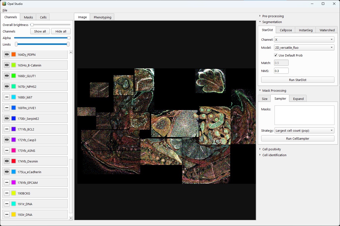
Opal Studio is a cross-platform viewer and analysis application for highly multiplexed imaging data, including Imaging Mass Cytometry (IMC), large OME-TIFF files, pyramid TIFF data, and SpatialData/Zarr V3 image directories.
The application combines fast multi-channel image rendering with practical workflows for preprocessing, segmentation, mask refinement, cell positivity, phenotype gating, clustering, and export.
Quick Start
Install From PyPI
Opal Studio needs Python 3.9 or 3.10 (TensorFlow 2.8, used by Mesmer, is not built for newer versions).
conda create -n opal-env python=3.9
conda activate opal-env
pip install opal-studio
opal-studio
Install From Source
git clone https://github.com/TristanWhitmarsh/opal-studio.git
cd opal-studio
conda create -n opal-env python=3.9
conda activate opal-env
pip install -r requirements.txt
pip install --no-deps -e .
python -m opal_studio
You can also launch an installed package with:
opal-studio
Create A Desktop Launcher
python -m opal_studio --create-launcher
On Windows this creates an Opal Studio.lnk shortcut on the desktop. On Linux it creates an OpalStudio.desktop launcher.
University Server / Darkroom Setup
On the server, Opal Studio is deployed as a source checkout installed into a conda env, so it can run the latest code rather than the last PyPI release. Install or update with:
# 1) Get / update the code
cd /home/tristan/Storage/scratch.space/users/tristan/opal-studio
git pull        # first time instead: git clone https://github.com/TristanWhitmarsh/opal-studio.git .

# 2) Activate the conda env
source /opt/conda/etc/profile.d/conda.sh
conda activate /home/tristan/Storage/scratch.space/envs/opal-env-j4

# 3) Install the pinned dependencies, then the package itself
PIP_REQUIRE_VIRTUALENV=0 pip install -r requirements.txt
PIP_REQUIRE_VIRTUALENV=0 pip install --force-reinstall --no-deps --no-build-isolation .

# 4) Create the desktop launcher
python -m opal_studio --create-launcher
Then double-click the Opal Studio icon on the desktop.
Notes:
pip install -r requirements.txtinstalls the full dependency stack; run it on the first install and wheneverrequirements.txtchanges. (Skipping it is why clustering, phenotyping, brightfield, or project-save features may report missing modules.)--force-reinstall --no-depsreinstalls only theopal_studiocode — picking up new code even when the version number is unchanged — without re-resolving dependencies.--no-build-isolationbuilds in place instead of copying the whole checkout to/tmp.- Do not launch with
python -m opal_studiofrom inside the checkout directory — that imports the checkout instead of the installed package. Use the desktop launcher, theopal-studioconsole script, or run from~.
Models
Model weights are not part of the package — they come to about 640 MB. They are downloaded automatically the first time they are needed:
- Opal Studio's own models (cell positivity, and the IMC / General segmentation
models) come from the
models-v1release of this repository. - StarDist, Cellpose and InstanSeg fetch their own pretrained models into their own caches, from their own sources.
Downloaded models are stored inside the installed package, in opal_studio/models/
under your environment's site-packages — next to the code, so nothing is left
elsewhere on the machine. Deleting the opal_studio folder deletes its models too.
pip only removes files it installed itself, so downloaded models survive
--force-reinstall, and pip uninstall leaves the models/ folder behind in
site-packages/opal_studio/. To fetch a model again, delete its folder there; it is
downloaded afresh the next time it is used.
Working offline, or on a cluster whose compute nodes have no internet: run
File → Download All Models once on a machine that is online (a login node, say).
To keep the models somewhere else — shared storage, for instance — set
OPAL_STUDIO_MODELS to a directory before starting Opal Studio:
export OPAL_STUDIO_MODELS=/home/tristan/Storage/scratch.space/opal-models
To use a model you trained yourself, place its folder under
<models>/<engine>/<name>/ (for example stardist/MyModel/) and it will appear in
that engine's model list. See MODELS.md for every model, its source and
its licence.
Supported Data
Opal Studio can open:
- OME-TIFF and TIFF image files, including multichannel and pyramidal data.
- SpatialData directories containing Zarr V3 image groups under
images/. - RGB-style TIFF series for brightfield/H&E viewing.
- Imported mask and cell label maps from OME-TIFF files.
- Phenotyping definitions from CSV files.
For OME-TIFF, channel names are read from OME metadata when available. For SpatialData, channel names are read from OME-Zarr metadata and can be enriched from extras/mcd_schema.xml when present.
Project Format (SpatialData)
File > Save Project writes the whole session as a spec-compliant SpatialData
store (Zarr v3, OME-NGFF 0.5-dev-spatialdata, store format 0.2). The stores
Opal writes can be opened directly by the spatialdata / squidpy ecosystem —
Opal does not depend on the spatialdata package, it drives the underlying
standards (Zarr v3, GeoParquet, AnnData) directly.
Segmentation masks become labels, hand-drawn regions become shapes, processed
channels and the generated brightfield become images, and the per-cell table
becomes tables (linked to the cell mask via region / region_key /
instance_key, so e.g. obs['region'].value_counts() gives cells-per-region).
project.zarr/
├── zarr.json                      # root group: spatialdata_attrs (v0.2) +
│                                  #   opal_studio {source_image, session} +
│                                  #   consolidated_metadata (flat list of all nodes)
│
├── images/
│   ├── zarr.json                  # group
│   ├── derived/                   # one OME-NGFF image element per key
│   │   ├── zarr.json              #   ome (multiscales; axes c,y,x; omero channels;
│   │   │                          #        coordinateTransformations) + spatialdata_attrs v0.3
│   │   └── 0/                     # scale-0 array (C,Y,X)
│   │       ├── zarr.json
│   │       └── c/ …               # chunk files  (c/<c>/<y>/<x>)
│   └── brightfield/
│       ├── zarr.json
│       └── 0/ { zarr.json, c/… }
│
├── labels/
│   ├── zarr.json                  # group
│   └── Cell Mask/                 # OME-NGFF label element (axes y,x, no channel)
│       ├── zarr.json              #   ome + spatialdata_attrs v0.3
│       └── 0/ { zarr.json, c/… }  # scale-0 array (Y,X)
│
├── shapes/
│   ├── zarr.json                  # group
│   └── Region 1/                  # ngff:shapes element
│       ├── zarr.json              #   encoding-type ngff:shapes, axes, transforms, v0.3
│       └── shapes.parquet         # GeoParquet (WKB polygons) — NOT a zarr node
│
├── tables/
│   ├── zarr.json                  # group
│   └── cells/                     # anndata-encoded Zarr-v3 group (ngff:regions_table v0.2)
│       ├── zarr.json              #   encoding-type anndata + region/region_key/instance_key
│       ├── X/            { zarr.json, c/… }        # array
│       ├── obs/                                    # dataframe
│       │   ├── zarr.json          #   column-order, _index
│       │   ├── _index/ { zarr.json, c/… }          # string-array
│       │   ├── cell_id/ { zarr.json, c/… }         # array
│       │   ├── area_px/ { zarr.json, c/… }         # array
│       │   └── region/                             # categorical
│       │       ├── zarr.json
│       │       ├── categories/ { zarr.json, c/… }  # string-array
│       │       └── codes/      { zarr.json, c/… }  # array
│       ├── var/         { zarr.json, marker/ }     # dataframe
│       ├── obsm/        { zarr.json, spatial/ }    # dict → arrays
│       ├── layers/      { zarr.json, positive/ }   # dict → arrays
│       ├── uns/                                    # dict
│       │   ├── zarr.json
│       │   └── spatialdata_attrs/ { region, region_key, instance_key }  # string scalars
│       ├── obsp/ varm/ varp/  { zarr.json }        # empty dict groups
│       └── raw/         { zarr.json }              # null
│
└── opal_aux/                      # Opal-private (ignored by SpatialData readers)
    ├── zarr.json                  # group
    └── cluster_labels/            # plain Zarr-v3 array (+ opal_key, opal_orig_shape attrs)
        ├── zarr.json
        └── c/ …
Notes:
images,labels,shapes, andtablesare standard SpatialData elements.opal_auxand theopal_studioroot attributes are Opal-private extras that SpatialData readers ignore.- Element directory names are filesystem-sanitized; the true layer name is preserved in each element's attributes.
- Only the root
zarr.jsoncarriesconsolidated_metadata; every other group omits it (so readers that open a sub-group directly fall back to a disk scan). shapes.parquetis a regular GeoParquet file, deliberately not part of the zarr hierarchy.- Element names must be unique across element types (a SpatialData requirement).
Application Layout
The main window has three working areas:
- Left panel: layer management for Channels, Masks, Positivity, Types, and Regions.
- Center tabs: Image, Phenotyping, Heatmap, t-SNE, and UMAP.
- Right panel: collapsible operation sections for Pre-processing, Segmentation, Mask Processing, Cell positivity, and Cell identification.
The status bar shows cursor position and the selected channel value while hovering over the image.
Core Functionality
Image Viewing
- Lazy, tiled rendering for large images.
- Pyramid-aware zooming so low-resolution levels are used when zoomed out.
- Background rendering with cached tiles to keep panning and zooming responsive.
- Mouse wheel zoom and left/middle mouse drag panning.
- Multi-channel compositing with per-channel color, alpha, and display limits.
- Global brightness control.
- Mask overlays with opacity and optional vector contours.
- Per-cell positivity overlays and phenotype/cluster type overlays.
Layer Management
The left panel separates generated and source layers:
- Channels: raw and processed image channels. Toggle visibility, change color, adjust alpha, adjust intensity limits, and show/hide all source channels.
- Masks: segmentation masks. Toggle raster overlay and contour visibility, adjust mask opacity, and delete generated masks.
- Positivity: marker positivity cell layers. Positive and negative cells share the same label map but use a positivity lookup table for display.
- Types: phenotype or cluster masks. Adjust shared type opacity and show/hide all type layers.
- Regions: hand-drawn polygon regions used for selected-region segmentation.
Generated processed channels, masks, positivity layers, type masks, and regions can be selected from this panel and reused by later steps.
Region Drawing
Use the Regions tab in the left panel to draw analysis regions:
- Click the draw button.
- Drag on the Image tab to trace a polygon.
- Release to create a region layer.
- Select the region layer before running segmentation in Selected region mode.
The simplification control reduces polygon point density. Existing region vertices can be dragged while draw mode is active.
Recommended Workflow
- Open data with
File > Open Image...orFile > Open SpatialData.... - Set up display in the Channels tab: choose visible markers, colors, alpha, brightness, and intensity limits.
- Preprocess channels if needed: merge markers, remove hot pixels, subtract background, rescale intensity, or create CLAHE-enhanced channels.
- Draw regions if you want to test or restrict analysis to a tissue area.
- Run segmentation on a full image, visible viewport, or selected region.
- Refine masks with size filtering, CellSampler mask fusion, or label expansion.
- Call marker positivity with AI or threshold-based per-cell intensity calls.
- Define phenotypes in the Phenotyping tab using marker positive/negative rules.
- Identify cells to create phenotype type masks, or run clustering to discover unsupervised cell populations.
- Inspect analysis views in Heatmap, t-SNE, and UMAP.
- Export results as OME-TIFF masks/cells, GeoJSON contours, and CSV phenotyping definitions.
File Menu
| Menu action | Purpose |
|---|---|
Open Image... |
Open OME-TIFF/TIFF image data. |
Open SpatialData... |
Open a SpatialData root directory. |
Load Masks... |
Import label masks from OME-TIFF/TIFF. |
Load Cells... |
Import cell/positivity label maps from OME-TIFF/TIFF. |
Load Phenotyping... |
Import phenotype definitions from CSV. |
Save Masks... |
Export mask layers as OME-TIFF. |
Save Cells... |
Export cell/positivity layers as OME-TIFF. |
Save Contours... |
Export selected mask/cell contours as GeoJSON. |
Save Phenotyping... |
Export phenotype definitions as CSV. |
Mask and cell OME-TIFF exports are written as CYX data with channel names preserved in OME metadata.
Pre-processing
Open Pre-processing in the right panel.
Merge
The Merge tab averages two selected image channels and creates a new processed channel named from the source pair.
Filter
The Filter tab creates a new processed channel from one source or processed channel. Available filters:
- Median: median filtering with a disk footprint.
- Opening: morphological opening for small-object/noise suppression.
- CLAHE: percentile normalization followed by contrast-limited adaptive histogram equalization.
- Subtract Background: Gaussian smoothing plus rolling-ball background subtraction.
- Remove Hotpixels: hot-pixel removal with threshold, pass count, and filter size controls.
- Intensity Rescale: percentile-based intensity rescaling.
Processed channels appear in the Channels tab and can be used for segmentation, positivity, and clustering.
Segmentation
Open Segmentation in the right panel. Choose a region mode, a target mode, and one segmentation engine.
Region Modes
- Full image: segment the entire image.
- Visible region: segment only the current canvas viewport, useful for fast parameter testing.
- Selected region: segment inside the selected polygon region. Only detections whose centroids fall inside the polygon are kept.
Target Modes
- New mask: create a new mask layer.
- Overwrite selected mask: update an existing selected mask. For region-based overwrite, existing cells in the affected area are removed and new detections are merged back in.
Engines
| Engine | Inputs and controls | Typical use |
|---|---|---|
| Watershed | One channel, Voronoi or Gaussian labeller, spot sigma, outline sigma, threshold, minimum mean intensity. | Fast classical nuclei/cell segmentation and parameter testing. |
| InstanSeg | One channel, model name, pixel size, optional hole filling and largest-component cleanup. | Fast learned nuclei/cell segmentation. |
| Mesmer | Nuclear channel, optional membrane channel, DeepCell/default or local .keras model, nuclear or whole-cell compartment, pixel size, watershed post-processing. |
Nuclear or whole-cell segmentation for multiplexed imaging. |
| StarDist | One channel, pretrained or local model, probability threshold, NMS threshold. | Nuclear segmentation with star-convex objects. |
| Cellpose | One channel, nuclei/cyto/cyto2 or local model, diameter, cell probability threshold, flow threshold. | Flexible cell or nuclei segmentation. |
| Omnipose | One channel, specialized Omnipose/custom model, diameter, mask threshold, flow threshold. | Bacteria, elongated objects, plant cells, worms, and other non-round shapes. |
Deep-learning engines run in a separate worker process to reduce TensorFlow/PyTorch conflicts. Models are downloaded on first use (see Models); your own model folders are auto-discovered under <models>/<engine>/.
Mask Processing
Open Mask Processing in the right panel.
| Tab | Function |
|---|---|
| Filter | Remove labels below a minimum area or above a maximum area. |
| Sampler | Merge multiple masks with CellSampler/Ubermasking. Strategies include largest cell count, highest Jaccard, and minimum area variance. |
| Expand | Expand labels by a chosen number of pixels. Binary Mask mode uses watershed-style separation lines; Label Map mode preserves integer labels with label expansion. |
Expanded binary masks keep their internal label map so threshold positivity and clustering can still operate per cell.
Cell Positivity
Open Cell positivity in the right panel after creating or importing a cell mask.
AI Positivity
The AI tab runs the packaged marker-positivity model against every non-mask image channel. For each channel it creates a Positivity layer that stores positive/negative calls per cell while preserving the original cell label IDs and contours.
Threshold Positivity
The Thresholds tab computes per-cell mean intensity for every image channel:
- Select a mask.
- Click Get Thresholds.
- Opal Studio computes per-cell means and an Otsu threshold for each channel.
- Positivity layers are created immediately for all channels.
- Use the channel dropdown, numeric threshold field, or threshold slider to adjust a channel interactively.
The count label shows positive cells over total signal-bearing cells for the selected marker.
Phenotyping And Cell Identification
Use the Phenotyping center tab to define cell types:
- Enter a cell type name and click Add Cell Type.
- Click table cells to cycle marker rules through blank,
Pos, andNeg. - Double-click a column header to rename a cell type.
- Right-click a column header to delete a cell type.
Then open Cell identification > Gating and click Identify Cells. Opal Studio combines the marker positivity layers with the phenotype table and creates one Type mask per matching cell type. Cells that do not match any defined type are added to an Unknown type mask.
Phenotyping definitions can be saved and loaded as CSV files.
Clustering
Open Cell identification > Clustering for unsupervised population discovery.
Inputs and options:
- Select the mask that defines individual cells.
- Choose which image or processed channels to include.
- Choose a normalization method: Yeo-Johnson, arcsinh, log-z, z-score, min-max, or none.
- Optionally enable PCA. If the PCA component count is blank, Opal Studio uses parallel analysis; DBSCAN uses PCA automatically.
- Choose a clustering method: Leiden, Louvain, PhenoGraph, FlowSOM, KMeans, Hierarchical, or DBSCAN.
Outputs:
- Type masks for each cluster, plus a grey Noise mask for DBSCAN noise when present.
- A Heatmap tab showing per-cluster mean channel intensity.
- t-SNE and UMAP plots colored by cluster.
- Clustering metrics including cell count, cluster count, PCA details, silhouette score, Davies-Bouldin index, Calinski-Harabasz index, and cluster sizes.
Cluster names can be edited in the Heatmap tab. Type mask color changes in the left panel are synchronized to the t-SNE and UMAP plots.
Model Selection Notes
For IMC datasets, start with models trained or tuned for IMC when available. If no custom model is available, a practical workflow is:
- Test quickly with Watershed or Visible region mode.
- Try InstanSeg or StarDist for nuclei-rich marker channels.
- Use Mesmer when nuclear and membrane/cytoplasm channels are available.
- Use Cellpose or Omnipose when object morphology differs from round nuclei.
- Refine with size filtering, CellSampler, and expansion before positivity or clustering.
Indicative speed from local high-resolution testing:
| Segmentation Engine | Approximate Speed |
|---|---|
| Watershed | 1 sec |
| InstanSeg | 10 sec |
| Mesmer | 26 sec |
| Cellpose | 14 sec |
| Omnipose | 25 sec |
| StarDist | 60 sec |
Typical IMC segmentation quality depends strongly on staining, tissue, resolution, and model weights. In earlier local testing, the rough ordering was:
StarDist > InstanSeg > Mesmer > Cellpose > Watershed > Omnipose
Treat this as a starting point rather than a rule.
Tips
- Use Visible region segmentation to tune parameters before running a full image.
- Use Overwrite selected mask when iterating on a segmentation to avoid clutter.
- Draw and select a region before using Selected region mode.
- Use processed channels as segmentation inputs when raw channels are noisy or low contrast.
- Keep one clean cell label mask for downstream positivity, phenotyping, and clustering.
- Save masks/cells before closing if you want to reuse generated label maps in another session.
License
Opal Studio is licensed under the MIT License with the Commons Clause.
- Free to use for research, internal analysis, and development.
- Free to inspect, modify, and build upon.
- You may not sell Opal Studio or offer it as a paid hosted service, paid software product, or commercial service whose value derives substantially from Opal Studio.
See LICENSE for the full license text.
1 maintainer

Download files
Download the file for your platform. If you're not sure which to choose, learn more about installing packages.
Source Distribution
Built Distribution
Filter files by name, interpreter, ABI, and platform.
If you're not sure about the file name format, learn more about wheel file names.
Copy a direct link to the current filters
File details
Details for the file opal_studio-0.1.4.tar.gz.
File metadata
- Download URL: opal_studio-0.1.4.tar.gz
- Upload date:
- Size: 1.4 MB
- Tags: Source
- Uploaded using Trusted Publishing? No
- Uploaded via:
twine/6.2.0 CPython/3.9.25
File hashes
| Algorithm | Hash digest | |
|---|---|---|
| SHA256 |
24dfe3b4f2c5fd678ab7a81ac0003f22d8bd8cd15e92b7d5b187a3f9a716c4bc
|
|
| MD5 |
2b29c5950e39070ab2771ff25db2d571
|
|
| BLAKE2b-256 |
9da1017fc189fde06cc85ae11310f418434b48f6b0c87b340b98bab390b7b2c5
|
File details
Details for the file opal_studio-0.1.4-py3-none-any.whl.
File metadata
- Download URL: opal_studio-0.1.4-py3-none-any.whl
- Upload date:
- Size: 1.4 MB
- Tags: Python 3
- Uploaded using Trusted Publishing? No
- Uploaded via:
twine/6.2.0 CPython/3.9.25
File hashes
| Algorithm | Hash digest | |
|---|---|---|
| SHA256 |
e5fee4c06df3bf1944f515bdae4a5e36776e1ee90881c30471fd513461500662
|
|
| MD5 |
d1eb924a156c22f38d9c4a1eba75d988
|
|
| BLAKE2b-256 |
88dacb92a661147029d84b6db8f0f79d561d524e56db779259135fb062e875ee
|














