
optika






A Python library for simulating optical systems, similar to Zemax.
optika computes the spectral response and resolution of an arbitrary optical system, and can optimize it using scipy.optimize.
Surfaces carry their own sag profile, aperture, material, and rulings, and are placed in global coordinates, so a system is an ordinary Python object that can be built, modified, and swept over programmatically.
Because every parameter can be an array from named-arrays, a whole configuration space of designs propagates through the raytrace at once, and an uncertain parameter carries its uncertainty through to the performance of the system.
More information is available in the documentation.
Installation
Optika can be installed using pip:
pip install optika
Features
- Sequential raytrace modeling of an optical system
- Stratified random sampling of input rays for faster convergence
- Image simulation of a given scene using an optical system
- A fast linear forward model approximating a raytraced system, for imaging many scenes without raytracing each one
- Spherical, conical, and toroidal surface sag profiles
- Circular, rectangular, and polygonal apertures
- Mirrors and arbitrary multilayer coatings
- Refractive glass materials with Sellmeier dispersion (e.g. N-BK7, F2)
- Diffraction gratings, with constant, polynomial, and holographic ruling spacing, and sinusoidal, square, rectangular, sawtooth, and triangular ruling profiles
- CCD/CMOS sensor simulation, including quantum efficiency, noise, and charge diffusion
- n-dimensional configurations of the optical system using named-arrays
- Uncertainty propagation using named-arrays
Key concepts
Surfaces are placed in global coordinates.
Unlike Zemax, where each surface is positioned relative to the one before it, an optika surface carries a transformation giving its position and orientation in the coordinate system of the whole instrument.
Moving one surface therefore does not move everything downstream of it.
The field of view and entrance pupil are computed, not specified.
The apertures of the surfaces determine them, so marking a surface with is_pupil_stop or is_field_stop is enough.
Rulings are a property of a surface.
A diffraction grating is an ordinary surface with a rulings field, so switching between ruling designs does not mean switching to a different type of surface.
Any parameter can be an array.
Giving a parameter an extra named axis sweeps the system over that axis, and every ray traced through it carries that axis along, which is how optika explores a configuration space without a loop.
An UncertainScalarArray parameter propagates its uncertainty through the raytrace by the Monte Carlo method.
Example Gallery
Simulate a Newtonian telescope
using optika
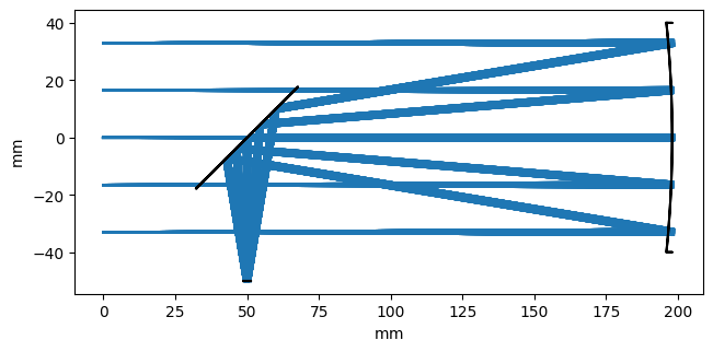
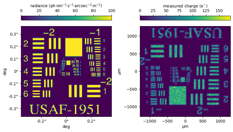
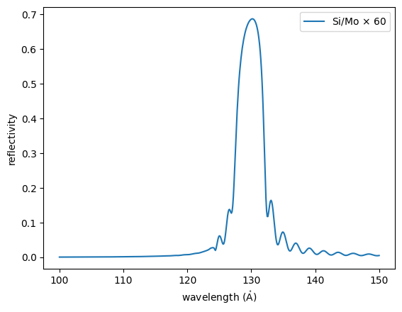
Compute the reflectivity of a multilayer mirror by specifying the materials and thicknesses of the layers.
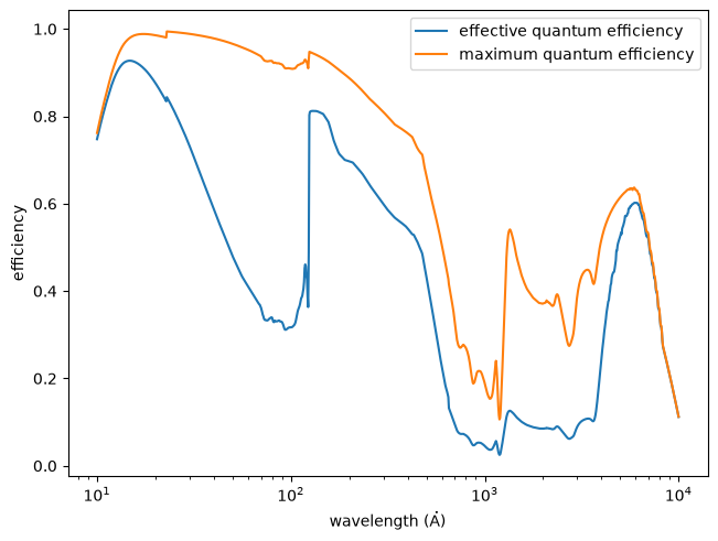
Model the quantum efficiency of a backilluminated CCD
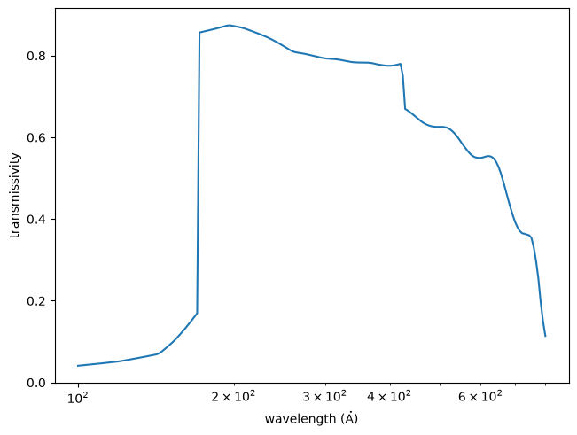
Compute the transmissivity of a thin filter, such as the aluminum filters used to reject visible light on solar instruments.
import matplotlib.pyplot as plt
import astropy.units as u
import named_arrays as na
import optika

# Define the wavelengths at which to compute the transmissivity
wavelength = na.geomspace(100, 800, axis="wavelength", num=201) * u.AA

# Compute the efficiency of a 100 nm layer of aluminum
reflectivity, transmissivity = optika.materials.multilayer_efficiency(
    wavelength=wavelength,
    layers=optika.materials.Layer(
        chemical="Al",
        thickness=1000 * u.AA,
    ),
)

# Plot the transmissivity, which drops sharply at the aluminum L edge
fig, ax = plt.subplots(constrained_layout=True)
na.plt.plot(wavelength, transmissivity.average, ax=ax, axis="wavelength");
ax.set_xscale("log");
ax.set_xlabel(f"wavelength ({wavelength.unit:latex_inline})");
ax.set_ylabel("transmissivity");
Development
Install the package in editable mode along with its test dependencies, and run the test suite using pytest:
pip install -e .[test]
pytest
This project is formatted using black, linted using ruff, and type-checked using mypy, all of which are checked by continuous integration:
black .
ruff check .
mypy optika
To build the documentation locally:
pip install -e .[doc]
sphinx-build docs docs/_build/html
1 maintainer

Metadata
1 maintainer
Release files for optika 2.3.0
For a detailed explanation of source distributions (sdists) and built distributions (wheels), please see the package formats documentation.
Source distribution (sdist)
| File | Size | Uploaded | |
|---|---|---|---|
| optika-2.3.0.tar.gz | 4.3 MB | Details |
Built distribution (wheel)
| File | Interpreter | ABI | Platform | Reset |
|---|---|---|---|---|
| optika-2.3.0-py3-none-any.whl | Python 3 | none | any | Details |
Total release size: 9.2 MB
Release files / optika-2.3.0.tar.gz
| Download URL | optika-2.3.0.tar.gz |
|---|---|
| Size | 4.3 MB |
| Tags | Source |
|
SHA-256 checksum How to use checksums |
9f727356151f7a9a57283bf50b4bafce6a61eda18b7625589230b236433c6128
|
|
BLAKE2b-256 checksum How to use checksums |
20bdec39e14d327fcb4dcb99dfe4fb9875d49d27ac613a44cb46d43ce561befe
|
| Upload date | |
|
Uploaded using Trusted Publishing? What is trusted publishing? |
No |
| Uploaded via |
twine/7.0.0 CPython/3.13.14
|
Release files / optika-2.3.0-py3-none-any.whl
| Download URL | optika-2.3.0-py3-none-any.whl |
|---|---|
| Size | 4.9 MB |
| Tags | Python 3 |
|
SHA-256 checksum How to use checksums |
72e6b11cdbb23bf617e71ef1065377f6244b1f154c62e7f0f18f457f2376314a
|
|
BLAKE2b-256 checksum How to use checksums |
28e0240473e6e62617515881c86c276229810ba23976abf57ae3ad152eadb782
|
| Upload date | |
|
Uploaded using Trusted Publishing? What is trusted publishing? |
No |
| Uploaded via |
twine/7.0.0 CPython/3.13.14
|














