
Organella: measuring label relationships in 3D
Organella measures segmented objects - 2D or 3D, one or a batch of them - and produces a single report you read in one standalone page: distributions, distances, contacts, and the objects themselves in 3D.
Open the viewer
Drop a report.parquet on it and every chart is drawn in your browser. Nothing is uploaded
and no server runs, so a report can be mailed to a collaborator with a link to that page.
Or read one that is already up: seven mouse β cells, from Müller et al. - FIB-SEM, eight structures, with its geometry beside it so the 3D sections draw.
An object is one segmented thing measured as a whole, given as a folder: a source image,
one mask that bounds the object, and the label/mask volumes inside it. For example, object can be a cell
bounded by its plasma membrane (--object-mask pm). Specifying the object bound is optional.
Everything inside is clipped to it by default, because a field of view often holds
neighbouring cells. --no-clip measures them anyway.
Screenshots from the reports
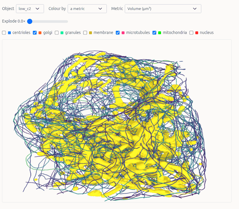 The object in 3D, from the geometry a --with-mesh run wrote. Structures switch on and off, colour by a metric, and explode pushes every instance out along its own direction from the centre. |
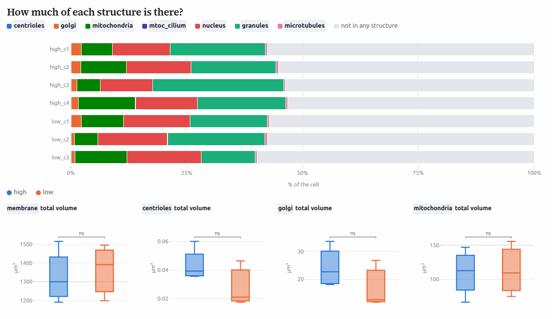 Composition, and groups compared. How much of each structure there is in each object, and a box per group with Mann-Whitney brackets between whatever the charts are faceted by. |
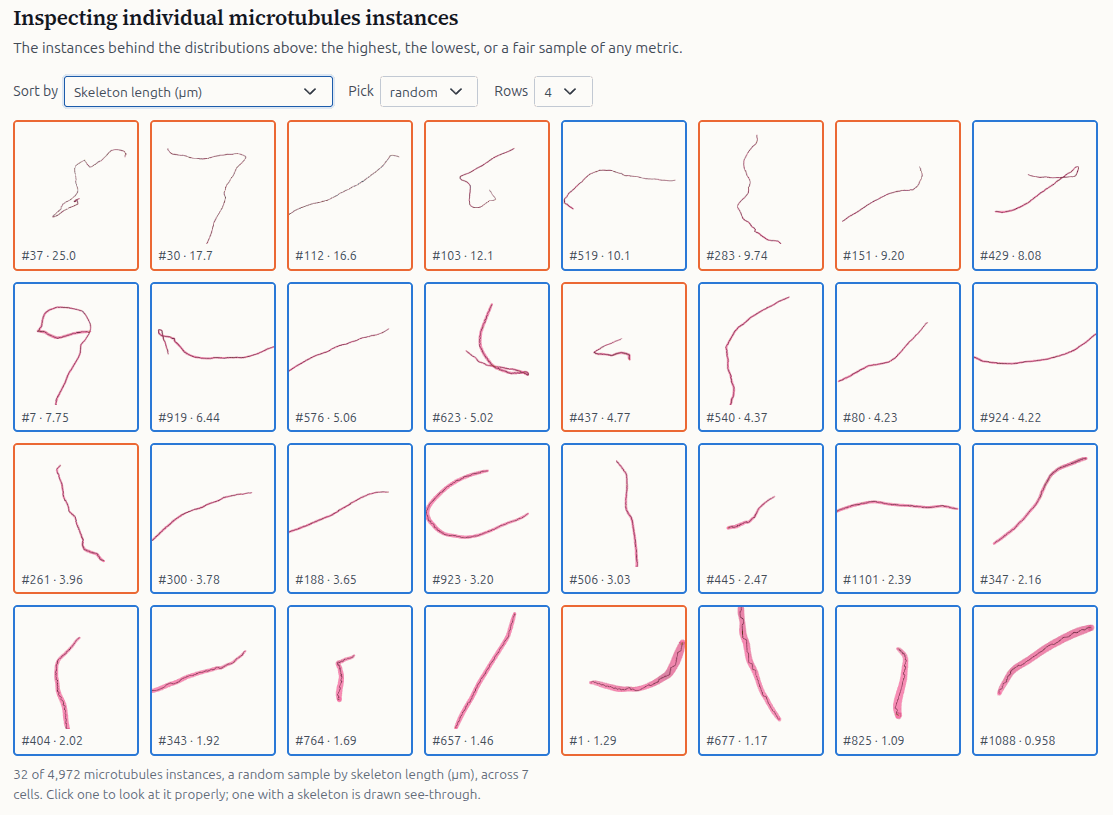 The instances behind a distribution: the highest, the lowest, or a fair sample of any metric. Click one to look at it properly. |
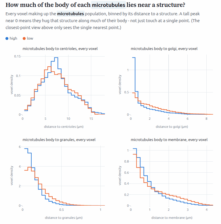 Every voxel, by distance. A structure's voxels binned by how far each one is from another structure, one panel per target. |
Workflow
- Organise your images in one of the input layouts.
organella dry-runto check what will be analysed.organella processto writereport.parquetand, with--with-mesh, the geometry.organella viewto open the report page on it.- Optionally import an object's geometry into Blender.
Try it
Install Organella:
pip install organella
Or with uv, which is quicker:
uv pip install organella.
Then test, measure, and view your label dataset:
organella dry-run experiment/
organella process experiment/ -o report.parquet --with-mesh
organella view report.parquet
The handful of arguments worth knowing from the start:
--object-mask pm |
the mask that bounds each object. It decides the origin of every distance and polarity, and everything inside it is clipped to it, so it is never guessed - dry-run lists the masks each folder has |
-p control -p treated |
subdirectories to import as groups. That grouping becomes the default comparison in every chart |
--voxel-size-um 0.1,0.02,0.02 |
needed when the images carry no calibration, since a size is never invented. y,x for a plane |
--skeletons mito,ER |
branches, length and tortuosity for the structures worth it. Opt-in: it is the most expensive thing in a run |
--entities mito,ER |
measure only these. Each entity is another full-size channel, so a subject carrying 117 structures needs this to fit in memory |
--with-mesh |
also write the geometry the 3D sections and Blender read, to <output>_meshes/ |
Every argument is listed under Parameters of process.
Check the input first. dry-run reads image headers only - no analysis, no output -
and prints per object the source image, the label and mask entities
found (* marks the object mask), and anything that looks wrong. Then which entities are
missing in which objects, and a suggested --max-workers. Exit code is 1 if any object
cannot be analysed.
control/cell_b
  source  sample_b.tif   [12.4 MB stacked]
  labels  mito
  masks   nucleus, pm*
  warn    ignored readme_overlay.tif: not <prefix>_<name>_label|labels|mask

===== 3 object folder(s) =====  (* = object mask)
  label:mito               2/3   ← missing in some objects
  mask:pm                  3/3
Reading the report
organella view report.parquet serves the report, its geometry and the page from one
localhost origin and opens it. Or open https://ida-mdc.github.io/organella/ and drop
report.parquet on it: the page parses the parquet in the browser, so nothing is uploaded and
no server runs.
The 3D sections need the geometry too. Press Add geometry and pick either the report_meshes folder or the
geometry.parquet files themselves; The organelle view command attaches them for you and you don't need to do anything else.
In the page, Charts switches every panel between boxes and histograms, and Significance puts Mann-Whitney brackets between the facets. Every column carries its own description in the report, so the page explains each metric under the chart of it.
A test compares objects, never instances. A box holds every instance of a facet - forty thousand granules across four cells - but the test behind its bracket is handed one number per object, the median of that object's instances, so the n it reports is a count of cells. Tested on the instances, any difference at all comes back as p < 0.001, because the test is told it has forty thousand independent samples when it has four: granules inside one cell share that cell's size, its fixation, its condition. Grouping the charts by object therefore leaves nothing to test - one cell per box - and no bracket is drawn, which the bar above the charts says while that grouping is on.
Every distance panel is drawn against chance. A run measures, per object and structure,
the distance to that structure from everywhere in the object, and the panels put it beside
what was measured: a dotted line at the distance half the object lies within (across the
boxes, or along the axis in histogram style), and a dotted curve beside the per-voxel
distributions. A population sitting below its line is closer to that structure than the
object's own shape puts anything; a population on top of the curve is placed no differently
from anything else in the object. That is a different statement from two conditions
differing, which is all a comparison between facets can say. --baseline-exclude decides
what is left out of that region.
The line allows for the fact that an instance has extent where a sample of the object has none - a granule reaches a structure from its surface, so its closest point is nearer than a point would be whatever else is true of it. The allowance is measured, not assumed: it is the gap between an instance's body average and its closest point, which the run records for every instance against every structure. For a sphere that gap is exactly its radius; for a filament along a structure it is far larger, and for one crossing it far smaller - so no shape is taken on faith. Each panel says how much was allowed for. The tip panels are read against the uncorrected line, because a tip is a point, and so are the per-voxel curves, which compare samples with samples.
Direction is read against a structure, not against the volume. Every polarity column is measured from the object mask's own centroid, which is the right origin but points wherever the volume happened to be oriented - so an azimuth means nothing from one object to the next. Pick a structure in Which way does each structure sit? and the direction from the centre to its centre becomes 0°: every angle is then measured against something inside the object and can be pooled. The section reports the angle per instance, the two collective measures per object - R, how tightly a structure's directions agree, and V, the same strength signed by whether it leans towards the reference (+1) or away from it (-1) - the angle against the distance from the centre, and one circular map per object. R and V are Polarity-JaM's polarity indices (Giese et al., Nat Commun 2025), so the numbers can be read beside that tool's, and its point about the statistics is taken: instances inside one object are not independent of each other, so the unit worth comparing between groups is one R and one V per object. This is a rotation of what was already measured, so it needs no re-run - but only what has a direction can be rotated, and a whole-structure mask has one centre and no more, so it appears as one reading per object rather than as a shape. The circular maps are one per object on purpose: the axis fixes 0°, but nothing in the data fixes the rotation about that axis, so which side of the circle a structure falls on is arbitrary.
A skeletonised structure is also measured at its tips. How far is each … end from other structures? is the distance of the nearest tip rather than of whichever part comes closest -
a filament can run past a structure along its whole length and end nowhere near it - and each
panel says what share of the population ends within one voxel of the structure, which is what
"connected to it" comes down to at a given voxel size.
Your input
Entity files must match <prefix>_<name>_label.tif (or _labels.tif) and
<prefix>_<name>_mask.tif, where <prefix> is the source image basename. The prefix is taken
off the front, so the entity name is whatever is left and may have underscores in it:
s0011_rib_left_11_mask.tif is the entity rib_left_11.
my_cell/
  sample.tif
  sample_mito_label.tif
  sample_nucleus_mask.tif
  sample_membrane_mask.tif
An object folder can sit on its own, in a flat batch (cells/cell_a/, cells/cell_b/), or in
a grouped batch (experiment/control/cell_a/, experiment/treated/cell_b/), where the group
folder is what -p imports.
Other formats. NIfTI (.nii, .nii.gz), NRRD and MetaImage are read through SimpleITK.
Their headers carry a reliable voxel size, which TIFF often does not; spacing is read as
millimetres, the convention every reader of these files uses.
Entities in a subfolder named by nothing but the structure - a segmentations/, masks/
or labels/ folder beside the source image. There is no prefix to strip, and label-or-mask
is read off the content rather than guessed from the name.
A remote store, read as a crop. A folder holding one source.json and no images names a
chunked store (N5 or Zarr, local or on S3), the arrays in it, and the window to read. A 512³
crop of OpenOrganelle's 122-gigavoxel HeLa cell is 0.64% of it, in under five seconds, at
full 4 nm resolution. Needs the remote extra: pip install 'organella[remote]'.
{
  "store": "s3://janelia-cosem-datasets/jrc_hela-2/jrc_hela-2.n5",
  "scale": "s0",
  "crop": "3712:4224,256:768,5760:6272",
  "source": "em/fibsem-uint16",
  "entities": { "mito": "labels/mito_seg", "er": "labels/er_seg" }
}
Output
report.parquet                            # rows per object, structure, instance and contact
report_meshes/<object>/geometry.parquet   # only with --with-mesh
Everything measured lands in report.parquet, as rows at four depths told apart by row_type:
row_type |
obs_level |
one row per |
|---|---|---|
object |
0 | object folder: extent, provenance, and the whole-object totals |
entity |
1 | structure, by name: volume, surface area, sphericity, instance counts |
instance |
2 | labelled instance: its own size, shape, polarity and nearest neighbour |
distance |
2 | instance × target structure: how far that instance is from it |
contact |
2 | touching pair of instances of one structure, with their gap |
Geometry goes beside the report rather than in it, because meshes would multiply the size of a
table every query loads. One geometry.parquet per object holds a surface per instance (an
outline, for a 2D object), the skeletons, and the touching pairs, so it stands on its own for
Blender and for a hosted copy. The object row records where, in mesh_geometry_file.
Commands
organella dry-run DIR |
what would be analysed, from headers only |
organella process DIR -o REPORT |
measure a batch, write the report |
organella mesh DIR -o OUTDIR |
geometry only, for a report you already have |
organella view REPORT |
serve the report, its geometry and the page, and open it |
organella page |
print the path of the standalone page |
organella colours REPORT PALETTE |
recolour a report in about a second |
organella describe REPORT TEXT |
say what the data is: credits, a citation, a licence. - reads it from standard input |
dry-run takes --object-mask NAME, to check every folder has it rather than only listing
what they have. view takes --port (default 8052) and --no-browser. mesh takes
-o, --out-dir for where to write <object>/geometry.parquet, plus the input, geometry and
run parameters below and --no-contacts.
Parameters of process
Input
-o, --output FILE |
where to write the report. Required |
-p, --paths TEXT |
subdirectory to import as its own group, repeatable. Becomes the default grouping in every chart |
--object-mask NAME |
the mask that bounds each object. Never guessed: it decides the origin of every distance and polarity. Left out, entities are measured where they lie |
--description TEXT |
what this data is and who it credits. It travels in the report, and the page shows it above the first section, so a report you send arrives with its provenance |
--object-noun WORD |
what one measured thing is called in the report, e.g. cell, or nucleus/nuclei for an irregular plural. Presentation only |
--voxel-size-um Z,Y,X |
voxel size in µm; y,x for a plane. Inferred from the source metadata when omitted, and refused rather than invented if there is none |
--entities NAMES |
measure only these, plus the object mask. Each entity is another full-size channel, so a 117-structure subject needs selecting down before it fits in memory |
--label-map FILE |
JSON of {"1": "liver"}, splitting one volume whose ids each mean a different structure into an entity per id. Only named ids become entities |
--label-map-entity NAME |
which entity --label-map splits. Needed only when a folder has more than one label entity, where leaving it out is an error rather than a guess |
--auto-label-masks |
promote masks with several connected components to label entities |
What gets measured
--no-clip |
measure outside the object mask too. Clipped to it by default, since that is what naming a bounding mask means |
--no-instances |
entity-level morphology only: no per-instance rows |
--no-contacts |
skip the contact rows |
--contact-max-um T |
largest gap between two instances of one structure that still counts as a contact. Default 0.5 |
--skeletons NAMES |
structures to skeletonise, for branches, length and tortuosity. Opt-in: it is the most expensive thing in a run, and a granule's skeleton is one branch the length of its diameter |
--max-skeleton-voxels N |
skip skeletons for instances above this voxel count. Default 500000 |
--polarity-spread |
also measure each instance's angular spread on the polarity sphere |
--distance-histograms |
also measure per-instance distance distributions, not just the minimum |
--baseline-exclude NAMES |
structures to leave out of the region every distance is read against. Each structure gets a chance distribution - its distance from everywhere in the object - and a measured distance only means something against that. Name the structures an instance could never sit inside, e.g. nucleus, so "closer than chance" is not decided by ground it was never free to occupy |
--colours FILE |
also --colors. JSON of {"mito": "#d62728"}. Lands in the report, so every chart draws that structure the same. Unnamed structures keep the built-in palette |
Geometry, all of it only with --with-mesh
--with-mesh |
also write per-object geometry for the 3D views and Blender. Goes to <output>_meshes/, never into the parquet |
--geometry-as NAME=KIND,... |
how a structure's surface is stored: mesh, ellipsoid or tube, e.g. vesicle=ellipsoid. Decided from the measured shape when unnamed - a round instance becomes a 60-byte ellipsoid, which is what makes tens of thousands drawable. No measurement changes; the surface is only ever drawn |
--mesh-max-vertices N |
most vertices one surface keeps; 0 lifts the cap. Default 200000. A decimation fraction bounds nothing: at 0.5 one ER sheet was still 2.87 million vertices and 86 MB |
--mesh-smooth-sigma SIGMA |
Gaussian sigma before marching cubes. Default 0.7; 0 disables |
--mesh-step-size N |
marching-cubes step size; 1 is full resolution. Default 2 |
--mesh-target-reduction F |
decimation fraction. Default 0.8, keeping ~20% of faces |
--mesh-level L |
iso-surface level on the signed distance field. Default 0 |
--mesh-surface-method |
marching-cubes or surface-nets. The dual method has ~30% less staircase noise, no fewer vertices, and is 66% slower |
--mesh-workers N |
processes meshing one object's instances. Default: the cores the object pool is not using |
--reuse-geometry |
keep any geometry.parquet an object already has. Meshing dominates a run, so a batch that died partway finishes in minutes |
The run
--max-workers N |
worker processes. Default: worked out from memory, since one object can need gigabytes |
--num-threads N |
kimimaro worker count. Default 1, because objects already run in parallel |
--resume |
skip objects an interrupted run already measured. Each object's rows go to <output>_parts/ as it finishes and are removed once the report is written |
Sharing a report
The geometry stays a folder of one file per object, so it travels with the report in one of two shapes:
- hand over
report.parquetand itsreport_meshes/folder, and the reader runsorganella view report.parquet - or upload the two together, unchanged, and open the page with
?data=<url of the parquet>. The geometry is looked for beside the parquet as<name>_meshes/, so there is nothing else to pass. If the files sit on a different origin than the page, that server has to allow cross-origin requests - GitHub Pages does, a barepython -m http.serverdoes not.
Development
uv venv --python 3.12 .venv
source .venv/bin/activate
uv pip install -e '.[test]'      # the suite needs pytest and duckdb
.venv/bin/python -m pytest
The report page is one file with no build step, edit
src/organella/report/organella_report.html
and reload the browser. The test suite runs it through
node - how a report is read into it, the maths its panels draw, the queries its 3D
sections build, and every section drawn against a stub DOM:
.venv/bin/python -m pytest tests/test_report_page.py
That harness never runs the real load path - DuckDB-WASM, the parquet read, WebGL - so a change to how the page opens a report has to be checked in a browser.
Blender
geometry_to_blender.py imports an object's geometry.parquet. It needs Blender with pandas
and pyarrow in Blender's own Python
(<blender>/python/bin/python3 -m pip install pandas pyarrow), and geometry from a 3D
object - a 2D object carries outlines, which the report's gallery draws and Blender has no use
for.
blender --background --python geometry_to_blender.py -- geometry.parquet [out.blend] [out.png]
Or open the script in Blender's Script Editor, set GEOMETRY_PATH (optionally OUT_BLEND,
OUT_RENDER) and run it with Alt+P.
1 maintainer

Download files
Download the file for your platform. If you're not sure which to choose, learn more about installing packages.
Source Distribution
Built Distribution
Filter files by name, interpreter, ABI, and platform.
If you're not sure about the file name format, learn more about wheel file names.
Copy a direct link to the current filters
File details
Details for the file organella-0.2.0.tar.gz.
File metadata
- Download URL: organella-0.2.0.tar.gz
- Upload date:
- Size: 739.2 kB
- Tags: Source
- Uploaded using Trusted Publishing? Yes
- Uploaded via:
uv/0.12.15 {"installer":{"name":"uv","version":"0.12.15","subcommand":["publish"]},"python":null,"implementation":{"name":null,"version":null},"distro":{"name":"Ubuntu","version":"24.04","id":"noble","libc":null},"system":{"name":null,"release":null},"cpu":null,"openssl_version":null,"setuptools_version":null,"rustc_version":null,"ci":true}
File hashes
| Algorithm | Hash digest | |
|---|---|---|
| SHA256 |
82b7c4c469d15f8939e9e1db44ffc8a1560809659308685869cce02db82de9e5
|
|
| MD5 |
13d7d5f1aacb1143247a8f56274f2ab3
|
|
| BLAKE2b-256 |
191df4f5c54e40d07b42be03491ea92175cd3660d41e28289f1a249afc77042f
|
File details
Details for the file organella-0.2.0-py3-none-any.whl.
File metadata
- Download URL: organella-0.2.0-py3-none-any.whl
- Upload date:
- Size: 305.3 kB
- Tags: Python 3
- Uploaded using Trusted Publishing? Yes
- Uploaded via:
uv/0.12.15 {"installer":{"name":"uv","version":"0.12.15","subcommand":["publish"]},"python":null,"implementation":{"name":null,"version":null},"distro":{"name":"Ubuntu","version":"24.04","id":"noble","libc":null},"system":{"name":null,"release":null},"cpu":null,"openssl_version":null,"setuptools_version":null,"rustc_version":null,"ci":true}
File hashes
| Algorithm | Hash digest | |
|---|---|---|
| SHA256 |
e63b2f8ee8336e866dd5675f2f33e3a21ffb8226ba0c2caa24e0a2f1a4b2b636
|
|
| MD5 |
7f0ba3aa2a39acb1e3d648117866a0a7
|
|
| BLAKE2b-256 |
f0d1499f7870fe2ef326b68897384574ea22a84dd2ce25274d0cb749265ea5c5
|














