







Contents
1. What this library does
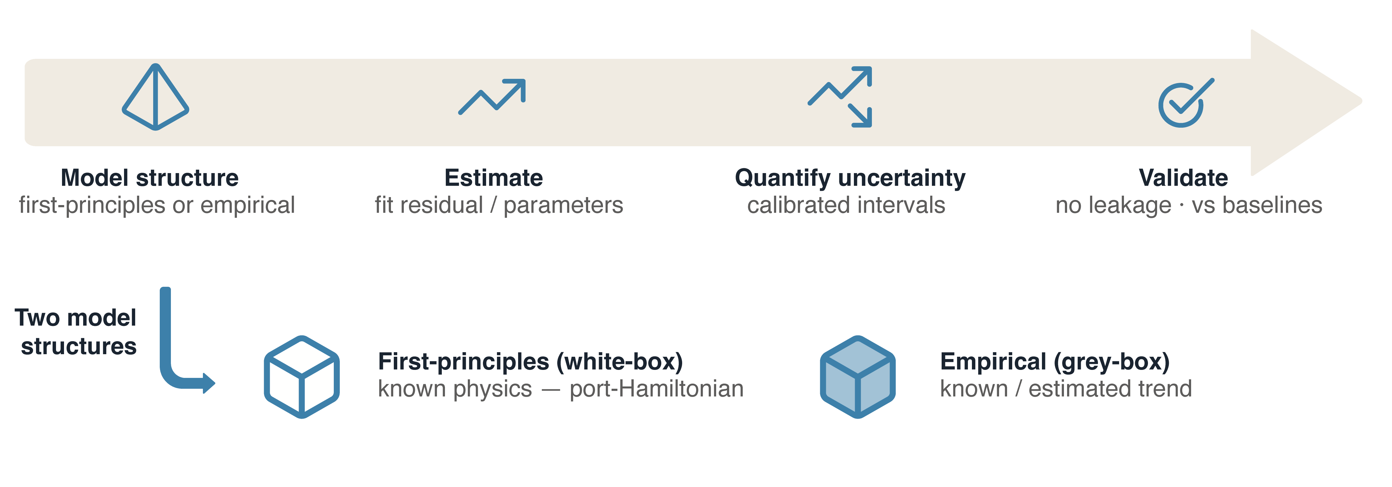
Otwin lets you write a lumped-parameter dynamic model of a physical system in energy form, simulate it, correct its state from sensor measurements, and measure how good its forecasts actually are.
It is intended for systems that store, move and dissipate energy: batteries and battery banks, electrical machines, hydraulic and pneumatic circuits, thermal networks, mechanical drivetrains, heat exchangers, pumped storage.
Otwin provides:
| A model class | A state-space model written in terms of stored energy, internal power routing, dissipation, and external ports |
| Numerical solvers | Including one whose discrete energy balance matches the continuous one |
| State estimators | Extended Kalman filter and moving-horizon estimation, to correct model state from measurements |
| Forecast validation | Out-of-sample partitioning, reference forecasters, skill scores, calibrated prediction intervals |
| Field data acquisition | SunSpec Modbus and Modbus TCP/RTU clients, for reading real equipment |
It is not a finite-element or CFD package, not an electrochemical simulator like PyBaMM, and not a replacement for Simulink. Section 9 states the scope limits explicitly.
2. Prerequisites
We suggest to use this library if you are comfortable with:
- Writing a system as a set of first-order ODEs,
dx/dt = f(x, u) - The idea of a state vector and an input vector
- Energy or power balances on a control volume or a circuit
- Basic Python: NumPy arrays, and defining a function or a class
You do not need:
- Prior knowledge of port-Hamiltonian systems (Section 4 explains the form from scratch)
- Lagrangian or Hamiltonian mechanics
- Machine learning
- Any knowledge of this library's internals
If you have written a state-space model in MATLAB or scipy.integrate, you have
enough background.
3. Installation and first run
The packages are not yet published on PyPI. Install from source:
pip install otwin
Then run a damped mass–spring–damper system:
import numpy as np
from otwin.model import PortHamiltonianSystem, integrate_phs

# States: x[0] = spring displacement q, x[1] = momentum p = m*v
# Parameters: stiffness k = 2 N/m, mass m = 1 kg, damping c = 0.3 N·s/m
osc = PortHamiltonianSystem(
    H      = lambda x: 0.5 * 2.0 * x[0]**2 + 0.5 * x[1]**2,   # potential + kinetic energy [J]
    grad_H = lambda x: np.array([2.0 * x[0], x[1]]),          # [force, velocity]
    J      = lambda x: np.array([[0.0, 1.0], [-1.0, 0.0]]),   # exchange between the two stores
    R      = lambda x: np.array([[0.0, 0.0], [0.0, 0.3]]),    # the damper
    g      = lambda x: np.array([[0.0], [1.0]]),              # external force applied to the mass
    n_states=2, n_inputs=1,
)

t = np.linspace(0, 20, 400)                   # 20 s, 400 points
u = np.zeros((400, 1))                        # no external force
sol = integrate_phs(osc, np.array([1.0, 0.0]), t, u)

E = np.array([osc.energy(x) for x in sol["x"]])
print(f"Initial energy: {E[0]:.4f} J")
print(f"Final energy:   {E[-1]:.4f} J")
print(f"Largest energy increase over any single step: {np.max(np.diff(E)):.2e} J")
The last line prints a number at or below 1e-9 J. That is the point of the
solver, and Section 5 explains why it matters.
To see the full workflow — reading a device, conditioning the signal, estimating state, forecasting, validating — run:
git clone https://github.com/otwin-core/otwin.git
cd otwin && pip install -e ".[dev]"
python examples/bess_end_to_end.py
That example simulates a grid-scale battery bank. It requires no hardware.
4. The model form
A system is described by four functions of the state, plus the state and input dimensions. The dynamics follow from them:
$$\frac{dx}{dt} = \bigl(J(x) - R(x)\bigr),\nabla H(x) + g(x),u \qquad\qquad y = g(x)^{\top},\nabla H(x)$$
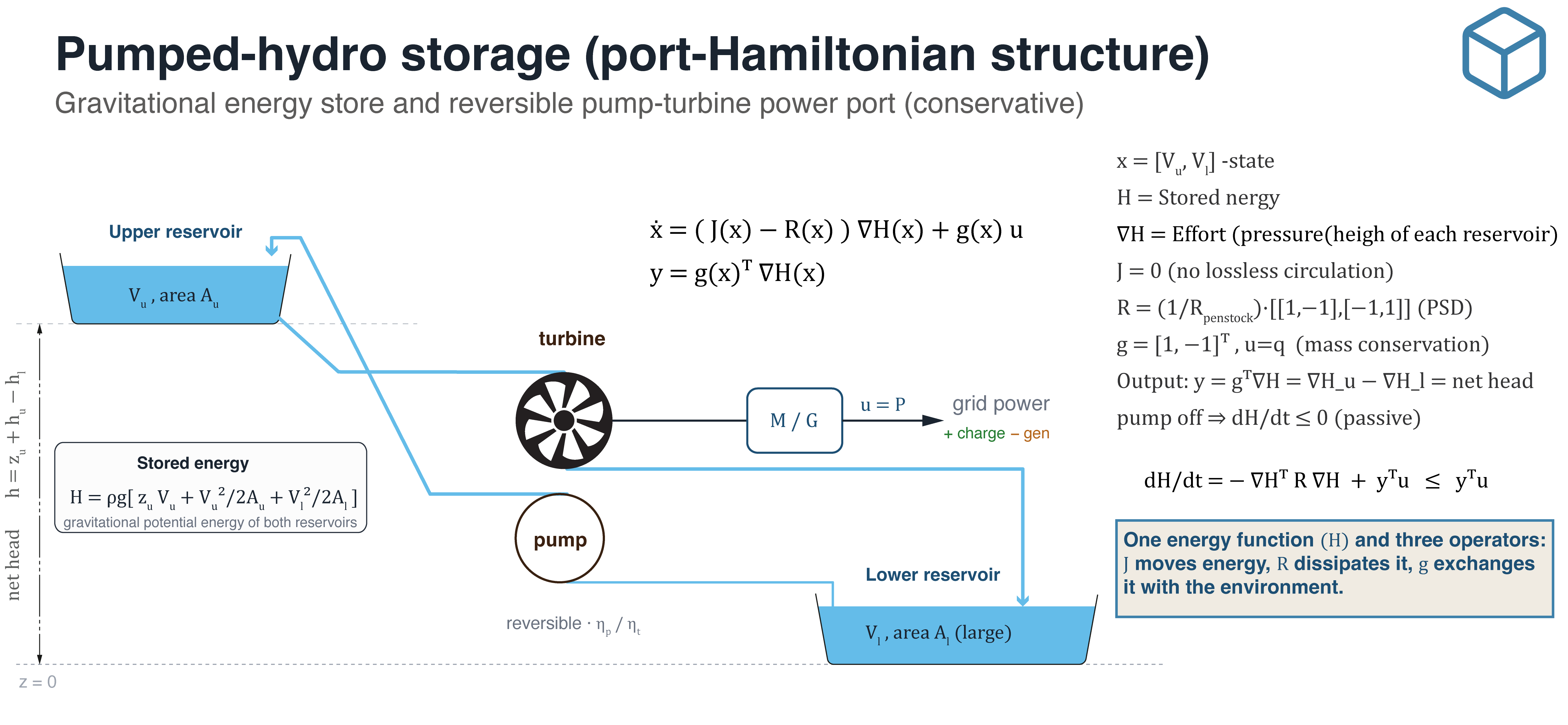
| Symbol | Meaning | Units | Example: a water tank |
|---|---|---|---|
| $x$ | state vector | varies | water height $h$ |
| $H(x)$ | total stored energy | J | $\tfrac{1}{2}\rho g A h^{2}$ |
| $\nabla H(x)$ | gradient of stored energy; the effort variables | V, N, Pa, K | pressure at the base |
| $J(x)$ | internal power routing between energy stores; must satisfy $J = -J^{\top}$ | — | zero (one store only) |
| $R(x)$ | dissipation; must be positive semidefinite | — | outlet orifice loss |
| $g(x)$ | external ports, where power crosses the system boundary | — | inlet pipe |
| $u$ | port input (flow variable) | m³/s, A, N | inlet flow rate |
| $y$ | port output (effort variable) | Pa, V, m/s | pressure at the inlet |
The product $y^{\top}u$ has units of power. This is the standard effort–flow pairing.
4.1 How this relates to what you already know
| Your background | The nearest concept you have already met |
|---|---|
| Mechanical | Bond graphs (Paynter 1959; Karnopp, Margolis & Rosenberg). $J$ is the junction structure with its transformers and gyrators; $R$ is the R-elements; $H$ is the C- and I-elements |
| Electrical | Equivalent-circuit models. $\nabla H$ are node voltages and branch currents; $J$ is the lossless interconnection; $R$ is the resistive network. Tellegen's theorem is the same statement |
| Chemical / process | An energy balance on a control volume, with the internal exchange terms separated from the irreversible loss terms |
| Control / telecom | Passive and dissipative systems in the sense of Willems (1972). $H$ is the storage function; $y^{\top}u$ is the supply rate |
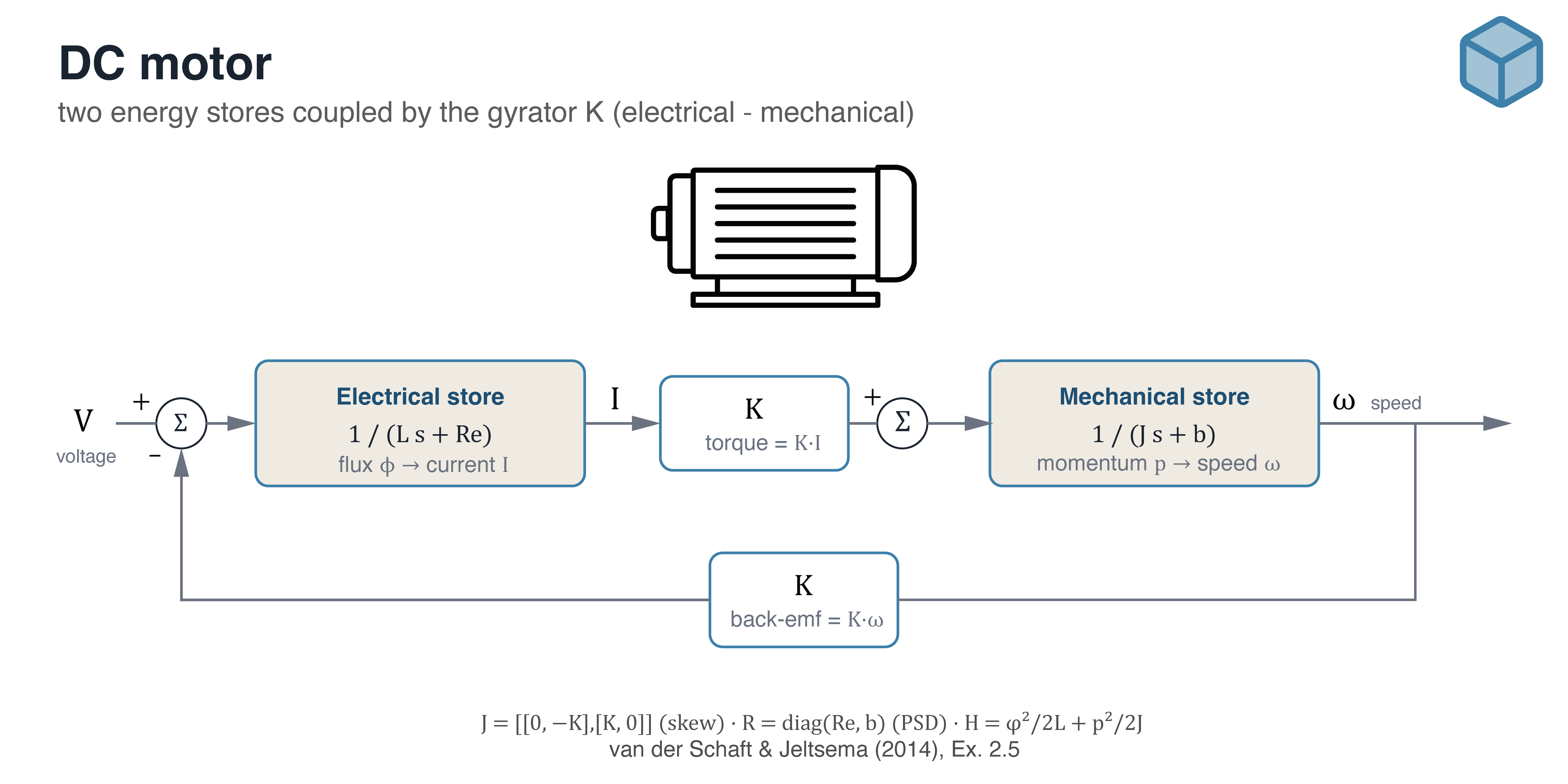
If you have drawn a bond graph or an equivalent circuit, you have already written $J$, $R$, $H$ and $g$ — the library only asks you to write them down separately instead of collapsing them into one right-hand side.
4.2 A complete worked model
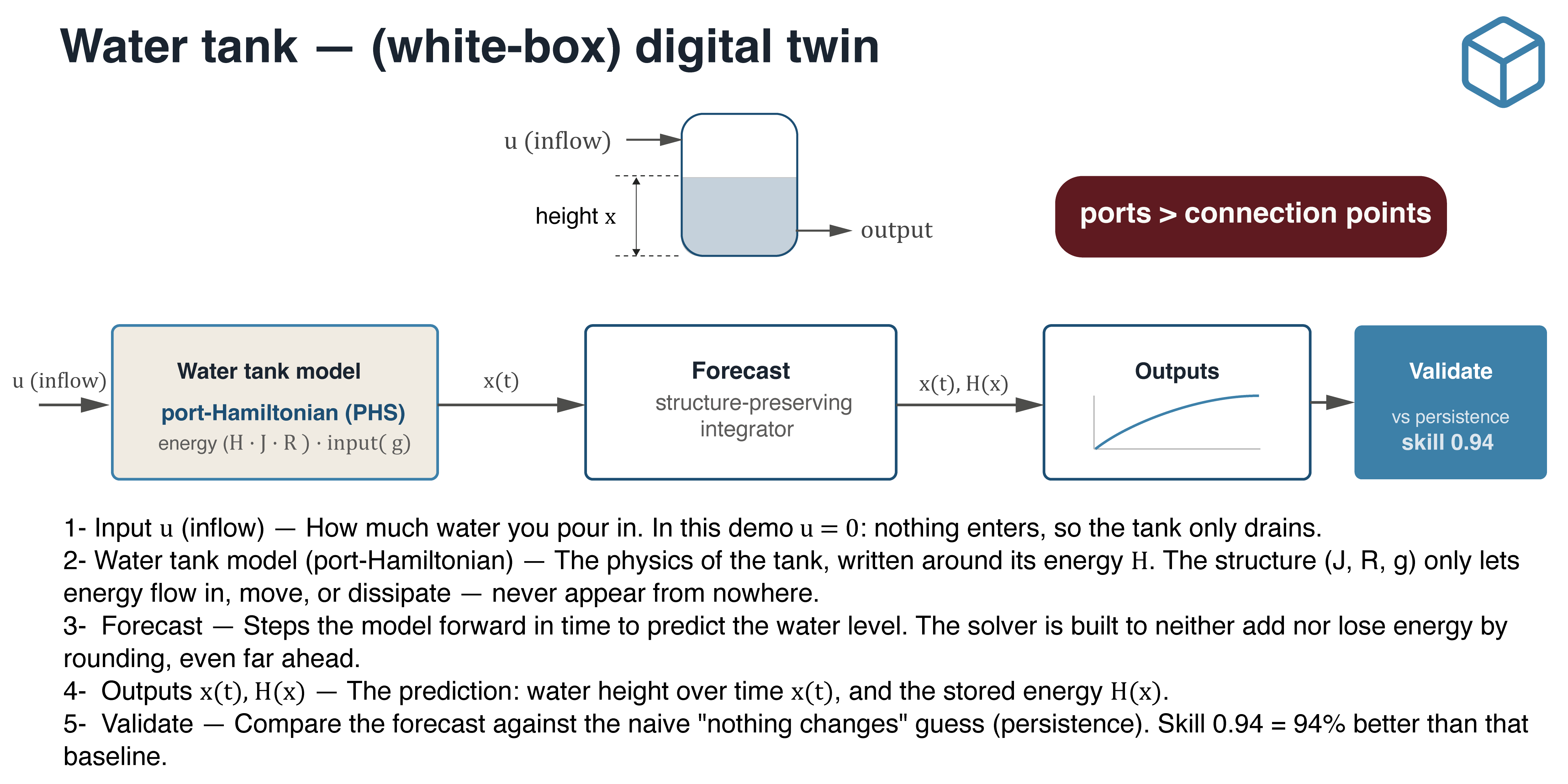
import numpy as np
from otwin.model import PortHamiltonianSystem

# Water tank, cross-section A, outlet orifice area a, discharge coefficient c_d.
A, a, c_d, rho, g_acc = 1.0, 0.1, 0.6, 1000.0, 9.81

tank = PortHamiltonianSystem(
    H      = lambda x: 0.5 * rho * g_acc * A * float(x[0])**2,     # [J]
    grad_H = lambda x: np.array([rho * g_acc * A * x[0]]),         # [Pa·m²] = [N]
    J      = lambda x: np.zeros((1, 1)),                           # one store: nothing circulates
    R      = lambda x: np.array([[c_d * a * np.sqrt(2 * g_acc / max(float(x[0]), 1e-9))
                                  / (rho * g_acc * A**2)]]),       # Torricelli outflow
    g      = lambda x: np.array([[1.0]]),                          # inlet
    n_states=1, n_inputs=1,
)

ok_J, dev_J = tank.check_structure(np.array([2.0]))["J_skew"]
ok_R, min_eig = tank.check_structure(np.array([2.0]))["R_psd"]
print(f"J skew-symmetric: {ok_J} (deviation {dev_J:.1e})")
print(f"R positive semidefinite: {ok_R} (min eigenvalue {min_eig:.1e})")
This model is available directly as otwin.model.water_tank.
5. What the two structural conditions give you
The two algebraic conditions, $J = -J^{\top}$ and $R \succeq 0$, have exactly two consequences. Both are provable, and both are worth understanding before you decide whether this library suits your project.
5.1 Bounded energy
Substituting the dynamics into $\dot{H} = \nabla H^{\top} \dot{x}$ and using $\nabla H^{\top} J \nabla H = 0$ (true for any skew-symmetric $J$):
$$\frac{dH}{dt} = -\nabla H^{\top} R, \nabla H + y^{\top} u ;\leq; y^{\top} u$$
With the ports open ($u = 0$), stored energy is non-increasing. This does not depend on the parameter values, the integration step size, or the simulation horizon. It is a consequence of the algebra, not of the fit.
Why this matters in practice. A model fitted to data reproduces the data it
was fitted to. Extrapolated beyond that range — a longer horizon, an untested
operating point — a purely fitted model can drift in a way that violates
conservation, and nothing in the model reports that it has. Here that specific
failure mode is excluded by construction. integrate_phs preserves the property
in discrete time as well: the worst per-step energy increase is bounded at
$10^{-9}$ of the initial value, against roughly $3\times10^{-5}$ for a standard
adaptive Runge–Kutta solver on the same problem.
What this does not give you. It does not make the model accurate. A model with the wrong parameters is still wrong; it is simply wrong without violating the energy balance. Accuracy is measured separately, in Section 6.
5.2 Composition
If two systems in this form are interconnected through their ports, the result is again a system in this form, and the energy bound holds for the assembly without refitting. This lets you build a subsystem model, validate it, and then use it inside a larger assembly — cell to module to string to bank, or component to loop to plant.
6. Validating a forecast
A model is not validated until its forecasts have been compared, out of sample, against a reference forecaster that is hard to beat.
from otwin.forecast import evaluate

report = evaluate(model, data, protocol="rolling_origin")
print(report)
Three conventions are built into the interface:
- Out-of-sample partitions by default. A random train/test partition on a
time series trains on Tuesday and Thursday to predict Wednesday. That
measures interpolation.
random_splitexists, warns, and marks the report. - A reference forecaster is required. The headline number is the skill score, model error divided by reference error. Persistence, drift, mean and seasonal-naive references are built in.
- The model is given history and a horizon, never the test values. The second argument to a forecaster is an integer number of steps.
$R^2$ is available but not shown first: on a trending series it commonly reads above 0.95 for a model that loses to repeating the last observed value.
For uncertainty, an interval is only meaningful once its coverage has been
measured on held-out data: a stated 90 % interval should contain the true value
about 90 % of the time. Interval.is_validated is False until that
measurement has been made.
7. Library structure
The modules follow the six data-processing blocks of ISO 13374 (Condition monitoring and diagnostics of machines), so the layout matches the reference architecture used in condition-monitoring practice.
| ISO 13374 block | Module | Contents |
|---|---|---|
| DA — Data Acquisition | otwin.io |
SunSpec Modbus (models 701, 702, 704, 713, 802–805), Modbus TCP/RTU, unit normalisation, device simulators for testing without hardware |
| DM — Data Manipulation | otwin.signal |
Resampling to a uniform grid, gap detection, out-of-order sample handling, measurement-coverage reporting |
| SD — State Detection | otwin.estimate |
Extended Kalman filter, moving-horizon estimation with state bounds, energy-consistent observer |
| HA — Health Assessment | otwin.model |
The model class, solvers, and a catalogue of worked physical models |
| PA — Prognostic Assessment | otwin.forecast |
Partitioning protocols, reference forecasters, error metrics, interval calibration |
| AG — Advisory Generation | otwin.advise |
Validity envelope: the operating range and horizon over which the model has been validated |
7.1 State estimation
otwin.estimate corrects model state from measurements. Two points a
control-systems reader will care about:
- The moving-horizon estimator accepts box constraints on the state. An extended Kalman filter will happily return a state of charge of 1.03; a constrained estimator will not.
- The energy-consistent observer limits any correction so that it does not increase stored energy beyond what the ports supplied. A standard Kalman correction can raise $H(x)$ with zero input, which breaks the property in Section 5.1. The limitation of this approach is documented in the docstring: with the ports open the allowed increase is zero, so a correction that only reflects an under-energetic prior is also rejected.
7.2 Validity envelope
otwin.advise.Envelope records the operating range and forecast horizon over
which a model was validated, and reports when a request falls outside it:
verdict = envelope.check(state=[0.42], horizon=900, manifest=twin)
print(verdict.explain())
# outside the validated envelope:
#   - horizon: beyond the validated forecast horizon (asked for 900, validated to 500)
This is the same discipline as stating the calibration range of an instrument. A reading outside the calibrated range is reported as such rather than returned as a number.
8. Suggested project topics
Each of these is a self-contained project. The first item lists what the library already provides; the second is what you would contribute.
Modelling and identification
- Model a physical system not yet in the catalogue — a heat exchanger network, a hydraulic actuator, a synchronous machine, a distillation column, a pneumatic circuit. Provided: the model class, structural checks, solvers. Yours: the four functions, parameter identification from data, and one result known in closed form (a steady state, an efficiency, a conservation law) used as a validation test.
- Grey-box parameter identification. Derive the structure from first principles, fit the unknown parameters to measured data, and report which parameters were estimated and how well they are identifiable.
Estimation and diagnostics
- Compare state estimators on a real asset. EKF against moving-horizon estimation on constrained states, using logged data. Provided: both estimators, the metrics. Yours: the data, the tuning study, the analysis of when the constraint handling matters.
- Sensor fault detection from the energy balance. Use the residual between
measured port power and modelled
dH/dtas a diagnostic signal for drift or bias in an instrument.
Forecasting
- Remaining useful life with calibrated intervals. Fit a degradation law, validate out of sample against a reference forecaster, and verify that the stated interval coverage is achieved. Aligns with ISO 13381-1.
- Compare a physics-based model against a purely data-driven one
out-of-sample and beyond the fitted range.
otwin-hybriddoes exactly this for a lithium-ion cell and is a template.
Instrumentation and integration
- Connect the library to real equipment. Read a PCS, inverter or BMS over SunSpec Modbus, condition the data, and drive a model in near-real time. Provided: SunSpec and Modbus clients, simulators. Yours: the register map for your equipment, the deployment, the results.
Numerical methods
- Implement and evaluate a structure-preserving integrator — the discrete gradient method is the obvious gap. Assessment is on energy conservation, not only on accuracy.
If you take one of these on, open an issue. The result is citable, and a model contributed to the catalogue carries your name.
9. Scope and limitations
- Lumped-parameter only. Ordinary differential equations in a finite state vector. No spatial discretisation, no PDEs, no finite elements.
- Not every system fits this form. Capacity fade, wear, fatigue and corrosion have no conserved energy function and no port through which power flows. Forcing them into an energy-balance frame is a modelling error. The library handles them separately, as empirical laws.
- Two communication protocols only. SunSpec Modbus and Modbus TCP/RTU. IEC 61850, IEC 60870-5-104 and DNP3 are out of scope: no permissively licensed Python implementation exists for them. Use a protocol gateway.
- Single maintainer, pre-1.0. Expect breaking API changes before version 1.0. Pin a version in your project.
- No production deployment yet. The library has been presented but not deployed on an operating asset. If you deploy it, please say so in an issue.
10. Repositories
| Repository | Contents |
|---|---|
otwin |
The library. Start here |
otwin-spec |
The specification and its type-test procedure: reference cases with closed-form answers, used to verify that an implementation is correct. Applies to implementations in any language |
otwin-hybrid |
A worked example in Python, Julia and R: predicting the end of life of a lithium-ion cell from the first 40 % of its life. Opens in Colab in one click |
Open contributor positions
otwin-spec verifies an implementation over a subprocess interface, so it can
test an implementation written in a language the Python library knows nothing
about. This makes a second-language implementation a well-defined piece of work
with an objective completion criterion: pass the test suite unmodified.
Julia and MATLAB implementations are both open. Scope is roughly a
thousand lines — the model class, an energy-consistent integrator, model
file I/O, and the test adapter. Open an issue titled Maintainer: <your name>,
or email javier@jmarin.info.
11. References
The formulation and methods are not original to this library. If you use it, cite the sources:
- van der Schaft, A. & Jeltsema, D. (2014). Port-Hamiltonian Systems Theory: An Introductory Overview. Foundations and Trends in Systems and Control.
- Willems, J. C. (1972). Dissipative dynamical systems. Archive for Rational Mechanics and Analysis, 45(5).
- Karnopp, D., Margolis, D. & Rosenberg, R. System Dynamics: Modeling, Simulation, and Control of Mechatronic Systems. Wiley.
- Ramírez, H., Maschke, B. & Sbarbaro, D. (2013). Irreversible port-Hamiltonian systems. Chemical Engineering Science, 89.
- Gneiting, T. & Raftery, A. E. (2007). Strictly proper scoring rules, prediction, and estimation. JASA, 102(477).
- ISO 13374 — Condition monitoring and diagnostics of machines: data processing, communication and presentation.
- ISO 13381-1:2015 — Condition monitoring and diagnostics of machines: prognostics.
Each repository carries a CITATION.cff.
12. Coming from another tool
- Simulink / Simscape — you already model as blocks exchanging power through ports. This is the same decomposition, written as four functions in a state space, with the conservation property following from the algebra rather than from careful block wiring.
- PyBaMM — PyBaMM models the electrochemistry of a cell. Otwin models the system around it and treats capacity fade as an empirical law, not an energy balance.
- scikit-learn — the workflow is the same shape: define a structure, fit, validate. The differences are that the structure comes from the physics, the partition is temporal, and a reference forecaster is required.
Licence
Apache 2.0.
1 maintainer

Download files
Download the file for your platform. If you're not sure which to choose, learn more about installing packages.
Source Distribution
Built Distribution
Filter files by name, interpreter, ABI, and platform.
If you're not sure about the file name format, learn more about wheel file names.
Copy a direct link to the current filters
File details
Details for the file otwin-0.2.0.tar.gz.
File metadata
- Download URL: otwin-0.2.0.tar.gz
- Upload date:
- Size: 230.4 kB
- Tags: Source
- Uploaded using Trusted Publishing? Yes
- Uploaded via:
twine/7.0.0 CPython/3.13.14
File hashes
| Algorithm | Hash digest | |
|---|---|---|
| SHA256 |
818d03378b4911a2ac44a574dcca784c034438543785c8ee5ca230246fd91a28
|
|
| MD5 |
b8fcb2dc724d5a109ae775b6b9157af2
|
|
| BLAKE2b-256 |
e79b0f2a231085ecb94f60d4824acd181266e12e1c95a32a20796b826b543cdd
|
Provenance
The following attestation bundles were made for otwin-0.2.0.tar.gz:
Publisher:
release.yml on otwin-core/otwin
-
Statement:
-
Statement type:
https://in-toto.io/Statement/v1 -
Predicate type:
https://docs.pypi.org/attestations/publish/v1 -
Subject name:
otwin-0.2.0.tar.gz -
Subject digest:
818d03378b4911a2ac44a574dcca784c034438543785c8ee5ca230246fd91a28 - Sigstore transparency entry: 2453342222
- Sigstore integration time:
-
Permalink:
otwin-core/otwin@b481591cd14ecfa6fba9fa35c2f486b8e75366f4 -
Branch / Tag:
refs/tags/v0.2.0 - Owner: https://github.com/otwin-core
-
Access:
public
-
Token Issuer:
https://token.actions.githubusercontent.com -
Runner Environment:
github-hosted -
Publication workflow:
release.yml@b481591cd14ecfa6fba9fa35c2f486b8e75366f4 -
Trigger Event:
push
-
Statement type:
File details
Details for the file otwin-0.2.0-py3-none-any.whl.
File metadata
- Download URL: otwin-0.2.0-py3-none-any.whl
- Upload date:
- Size: 156.7 kB
- Tags: Python 3
- Uploaded using Trusted Publishing? Yes
- Uploaded via:
twine/7.0.0 CPython/3.13.14
File hashes
| Algorithm | Hash digest | |
|---|---|---|
| SHA256 |
0455b0885c6f0f2697610e2ca86f43f7079e503d71bad1467aa1cf8957dd98ca
|
|
| MD5 |
6020c52a60d07ed06ee0df5e86e9332f
|
|
| BLAKE2b-256 |
8067e9f98b4d3b04eeebbd1fc12f3e68c4115055f8d53979a5bc7fde860b27a1
|
Provenance
The following attestation bundles were made for otwin-0.2.0-py3-none-any.whl:
Publisher:
release.yml on otwin-core/otwin
-
Statement:
-
Statement type:
https://in-toto.io/Statement/v1 -
Predicate type:
https://docs.pypi.org/attestations/publish/v1 -
Subject name:
otwin-0.2.0-py3-none-any.whl -
Subject digest:
0455b0885c6f0f2697610e2ca86f43f7079e503d71bad1467aa1cf8957dd98ca - Sigstore transparency entry: 2453342254
- Sigstore integration time:
-
Permalink:
otwin-core/otwin@b481591cd14ecfa6fba9fa35c2f486b8e75366f4 -
Branch / Tag:
refs/tags/v0.2.0 - Owner: https://github.com/otwin-core
-
Access:
public
-
Token Issuer:
https://token.actions.githubusercontent.com -
Runner Environment:
github-hosted -
Publication workflow:
release.yml@b481591cd14ecfa6fba9fa35c2f486b8e75366f4 -
Trigger Event:
push
-
Statement type:







