
A Robust Futures CryptoCurrency Backtesting Library.

Project description
Overfitting (Futures Backtesting)
Overfitting simulates a realistic crypto futures trading environment including
- Liquidation, Margin, Leverage for stress testing
- Multiple Currency Trading (e.g., backtesting BTC PERP & ETH PERP at the same time)
- Four Different Order Types: LIMIT, MARKET, STOP_LIMIT, STOP_MARKET
- Slippage/Commission Setting
Installation
$ pip install overfitting
Usage
import pandas as pd
from overfitting import Strategy
from overfitting.indicators import SMA

def load_data():
    df = pd.read_csv('./data/BTCUSDT.csv')
    benchamrk_df = pd.read_csv('./data/BTCUSDT.csv') # BTC buy and Hold
    df['timestamp'] = pd.to_datetime(df['timestamp'], unit='ms')
    df.set_index('timestamp', inplace=True)

    start_time = pd.to_datetime('2023-01-01 00:00:00')
    df = df.loc[start_time:]

    return df, benchamrk_df

class MyStrategy(Strategy):
    def init(self):
        self.asset = 'BTC'
        self.set_leverage(self.asset, 1)

        self.sma_short = self.indicator(SMA, self.asset, window=20)
        self.sma_long = self.indicator(SMA, self.asset, window=50)

    def next(self, i):
        if i == 0:
            return

        sma_short = self.sma_short[i]
        sma_long = self.sma_long[i]
        previous_sma_short = self.sma_short[i - 1]
        previous_sma_long = self.sma_long[i - 1]

        if (
            pd.isna(sma_short) or pd.isna(sma_long) or
            pd.isna(previous_sma_short) or pd.isna(previous_sma_long)
        ):
            return

        position = self.get_position(self.asset)

        # Golden cross (entry)
        if previous_sma_short <= previous_sma_long and sma_short > sma_long and position.qty == 0:
            open_price = self.open(self.asset, i)
            lot_size = self.get_balance() // open_price
            self.limit_order(self.asset, lot_size, open_price)

        # Death cross (exit)
        if previous_sma_short >= previous_sma_long and sma_short < sma_long and position.qty > 0:
            self.market_order(self.asset, -position.qty)

price_df, benchmark_data = load_data()
strategy = MyStrategy(
    data={"BTC": price_df},
    benchmark=benchmark_data, # Default = None Optional
    initial_capital=100_000, # Default Optional
    commission_rate=0.0002, # Default Optional
    maint_margin_rate=0.005, # Default Optional
    maint_amount=50  # Default Optional
)
returns = strategy.run()
strategy.plot(returns)
Results
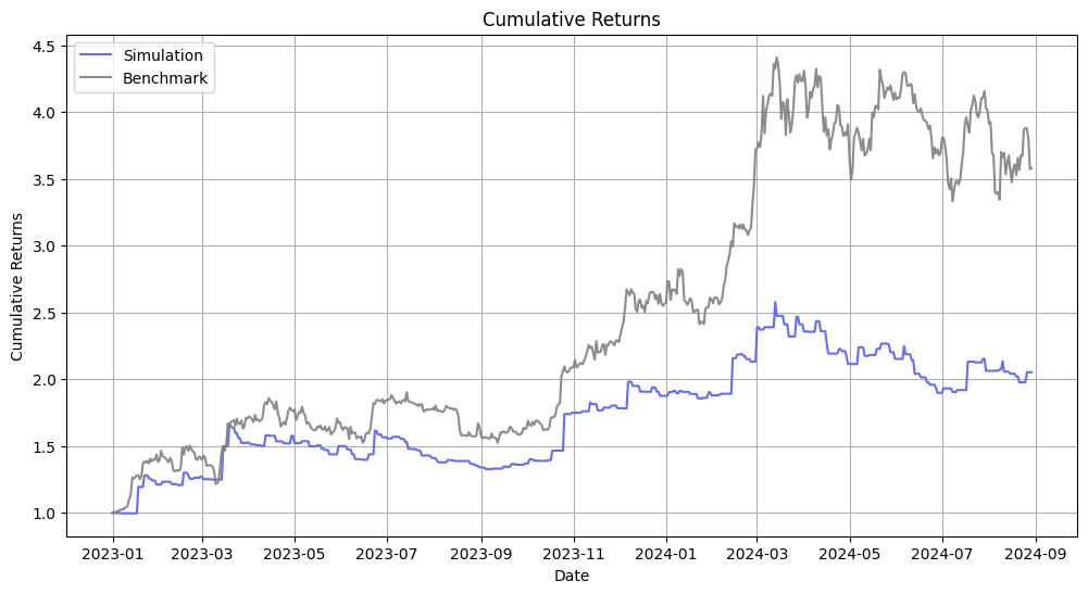
Performance Summary
Number of Years               1.66000000
Start Date           2023-01-01 00:00:00
End Date             2024-08-29 00:00:00
Initial Balance         100,000.00000000
Final Balance           205,328.91120000
CAGR                          0.52684228
Cumulative Return             2.05328911
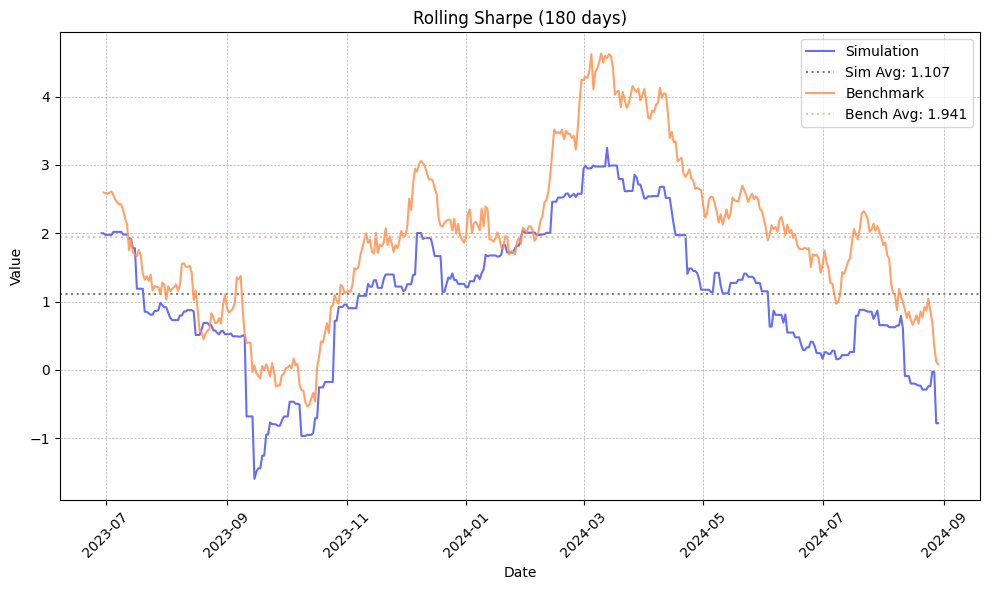
Sharpe Ratio                  1.24678659
Sortino Ratio                 3.54979579
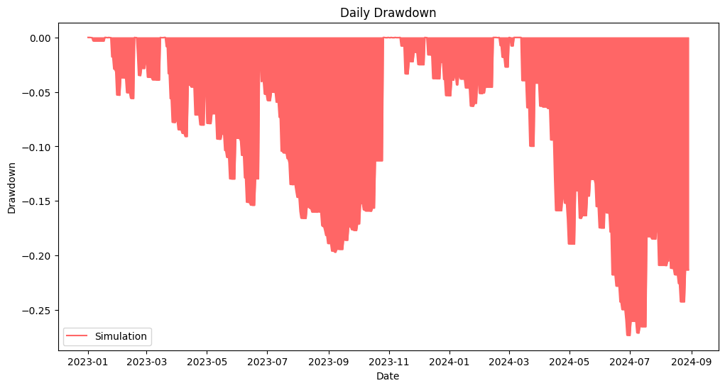
Max Drawdown                 -0.26332695
Daily Value At Risk          -0.04147282
Skew                          0.44515551
Kurtosis                      2.66444346
Total Trades                182.00000000
Winning Trades               69.00000000
Losing Trades               113.00000000
Win Rate (%)                 37.91208791
Gross Profit            399,044.19246000
Gross Loss             -293,715.28126000
Net Profit              105,328.91120000
Avg Return (%)                0.38834383
Avg Profit (%)                3.54140613
Avg Loss (%)                 -1.53697740
  Net drawdown in %  Peak date Valley date Recovery date Duration
0         26.332695 2024-03-13  2024-06-30           NaT      NaN
1         19.678014 2023-03-20  2023-09-07    2023-10-26      159
2          6.297244 2023-12-07  2024-01-24    2024-02-14       50
3          5.585429 2023-01-22  2023-02-14    2023-02-17       20
4          3.898568 2023-02-17  2023-03-11    2023-03-15       19
5          3.336877 2023-11-12  2023-11-18    2023-12-07       19
6          2.699556 2024-02-20  2024-02-26    2024-03-01        9
7          0.767196 2024-03-01  2024-03-03    2024-03-06        4
8          0.324161 2023-01-03  2023-01-07    2023-01-18       12
9          0.019817 2023-11-03  2023-11-04    2023-11-07        3
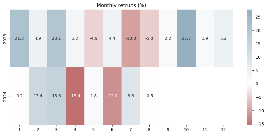
Performance Visualizations Examples
Liquidation Handling
The liquidation logic is based on isolated margin mode:
- Initial Margin = Entry Price × Quantity / Leverage
- Maintenance Margin = Entry Price × Quantity × Maintenance Margin Rate − Maintenance Amount
- Liquidation Price is then calculated based on whether the position is long or short.
- Long Position Liquidation Price => Entry Price - (Initial Margin - Maintenance Margin)
- Short Position Liquidation Price => Entry Price + (Initial Margin - Maintenance Margin)
When the price crosses the calculated liquidation level, the position is force-closed and the entire margin is lost.
Supported Order Types
Supports four order types: LIMIT, MARKET, STOP LIMIT, and STOP MARKET. Each behaves according to standard trading conventions.
[NOTE] Rules
- For MAKRET Orders, the system will automatically execute the trade with "open" price.
- For STOP Orders, the system will automatically trigger the order when:
- Long: Price (High) >= Stop Price
- Short: Price (Low) <= Stop Price
- Stop Order Immediate Rejection Rule: If a STOP LIMIT or STOP MARKET order would trigger immediately upon creation (because the current price already breaches the stop price), the system rejects the order with "STOP order would Immediately Trigger" message.
limit_order(symbol: str, qty: float, price: float)
market_order(symbol: str, qty: float)
stop_limit_order(symbol: str, qty: float, price: float, stop_price: float)
stop_market_order(symbol: str, qty: float, stop_price: float)
Multiple Currency Backtesting
You can simply test multiple currencies by passing data as dict[str, pd.DataFrame]. For examples, please refer to "multi_currency_sma_corss.ipynb" under "examples" folder.
Upcoming Features
- Parameter Optimizer
A simple optimizer to help find the best-performing strategy parameters (like SMA windows, thresholds, etc.) based on backtest results.
💡 Got feedback or suggestions? Feel free to open an issue or contribute via pull request.
Release history Release notifications | RSS feed


Download files
Download the file for your platform. If you're not sure which to choose, learn more about installing packages.
Source Distribution
Built Distribution
Filter files by name, interpreter, ABI, and platform.
If you're not sure about the file name format, learn more about wheel file names.
Copy a direct link to the current filters
File details
Details for the file overfitting-0.4.2.tar.gz.
File metadata
- Download URL: overfitting-0.4.2.tar.gz
- Upload date:
- Size: 28.3 kB
- Tags: Source
- Uploaded using Trusted Publishing? No
- Uploaded via: twine/6.1.0 CPython/3.13.3
File hashes
| Algorithm | Hash digest | |
|---|---|---|
| SHA256 |
7c025118395ac47a9254f2116efc71101347252b0690fc04d26e1cf1135b1f0f
|
|
| MD5 |
d4dc9f4bb6471470c92a6be01cd0173c
|
|
| BLAKE2b-256 |
2fbe42166463607333e1087b99d9d0cd67c730cce9eb89ccb1679f0bc46e27ae
|
File details
Details for the file overfitting-0.4.2-py3-none-any.whl.
File metadata
- Download URL: overfitting-0.4.2-py3-none-any.whl
- Upload date:
- Size: 28.6 kB
- Tags: Python 3
- Uploaded using Trusted Publishing? No
- Uploaded via: twine/6.1.0 CPython/3.13.3
File hashes
| Algorithm | Hash digest | |
|---|---|---|
| SHA256 |
f4a4f8953484677bbc63d5b62b114dc38fc412fe95743f52f9ab653f06e86fac
|
|
| MD5 |
473c5c5b93ec057124082db0baf6521f
|
|
| BLAKE2b-256 |
d44b00febe7f3189229b6c14129436cecfd22f6e1a07d324fe86bf806f050653
|






