
p3k14c-py
Python package for the p3k14c global archaeological radiocarbon database with comparisons to paleoenvironmental datasets.
Datasets were sourced from the PAGES People3000 Archaeological Radiocarbon, NOAA GISP2, PANGAEA, and Neotoma databases, which are all in the public domain.
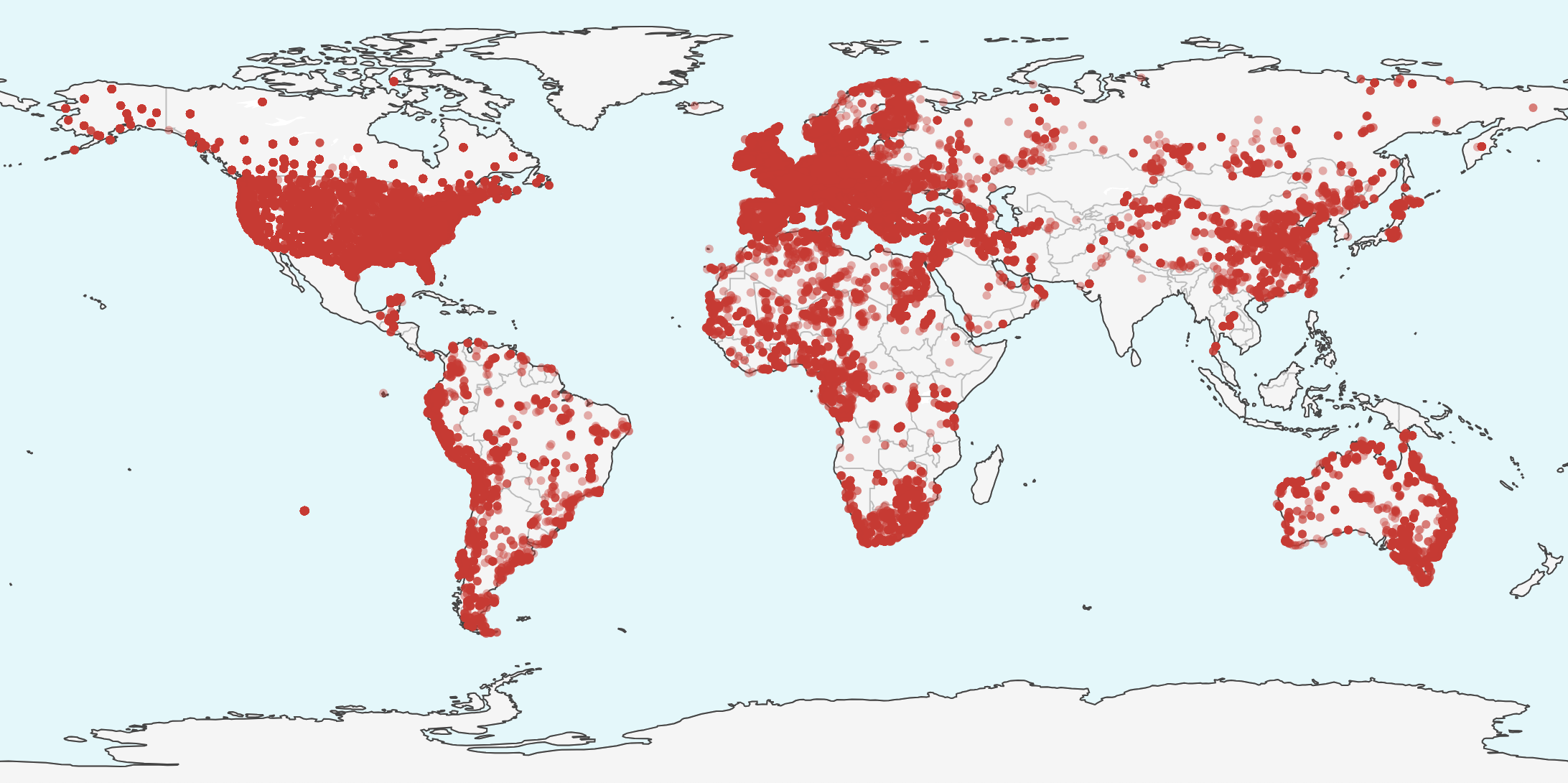
Before Running
For more information on the database and original scrubbing methodology, see the official Scientific Data publication.
See the official p3k14c GitHub page for the original implementation using the R Language.
The cleaned and calibrated dataset is available in the GitHub repository (see Datasets/p3k14c_pristine_dates.csv). You can bypass the finicky cleaning and calibrating process entirely.
Introduction
The PAGES People3000 Archaeological Radiocarbon Database (p3k14c) is a comprehensive, global database of archaeological radiocarbon dates. The raw data, however, is uncalibrated and can be messy. This can be daunting for researchers new to coding or who want to reproduce findings. The p3k14c project originally released code in R to help researchers tackle the dataset, relying heavily on great R packages like rcarbon.
While R is a fantastic language for statistical analysis and has been heavily adopted by archaeologists, it has limitations in areas pertaining to data engineering, complex GIS integration, machine learning scalability, and large-scale data handling.
This repository bridges that gap. p3k14c-py provides detailed Python scripts for the calibration, filtering, and analysis of the p3k14c dataset, enabling better integration into the broader Python data science community.
Installation and Requirements
The recommended way to use this repository is now the paleopy Python package (see below), which supersedes the standalone scripts in Scripts/. To install it from PyPI:
pip install "paleopy[all]"
This installs the core dependencies (numpy, pandas, scipy, matplotlib, requests) plus every optional extra: calibration (iosacal, radiocarbon), stats (scikit-learn, seaborn), mapping (cartopy), text (ftfy), progress (tqdm). Install a subset instead if you only need part of the pipeline, e.g. pip install "paleopy[calibration]".
To work on the code itself, clone the GitHub repository and install it in editable mode from the repository root:
pip install -e ".[all,dev]"
paleopy downloads some reference data on first use (the IntCal20 calibration curve, proxy records, and Natural Earth land geometry for maps) and always verifies HTTPS certificates. If you installed Python from python.org on macOS and see an SSL: CERTIFICATE_VERIFY_FAILED error, run the Install Certificates.command script in your /Applications/Python 3.x/ folder once, then try again.
If you'd rather run the original standalone scripts directly (see Scripts/, kept for reference — see the note below), install the same libraries manually:
pip install pandas scipy numpy matplotlib seaborn scikit-learn iosacal radiocarbon cartopy tqdm ftfy requests
The paleopy Package
The functionality of all seven scripts below has been ported into an installable Python package, paleopy (see src/paleopy/), with one console script per original script:
| Console script | Replaces | Purpose |
|---|---|---|
paleopy-clean |
01_Data_Cleaning_and_Prep.py |
Clean/scrub the raw p3k14c dataset |
paleopy-calibrate |
02_Calibrating.py |
IOSACal radiocarbon calibration |
paleopy-summary |
03_SummaryStats.py |
Summary statistics + dashboard |
paleopy-spd |
04_SPD.py |
SPD paleodemography pipeline |
paleopy-climate |
05_Human_Climate_Interaction.py |
Human-climate comparison |
paleopy-ccsi |
06_Composite_Human_Environment.py |
Composite Climate Stress Index (PCA) |
paleopy-kde |
07_KDE.py |
Spatial KDE visualizer |
Each console script accepts --input/--outdir plus named flags for the settings that used to be hardcoded module-level constants in the scripts (e.g. --site-name, --site-lat, --site-lon, --time-min, --time-max). Run any of them with --help for the full option list. For example, to reproduce the Çatalhöyük SPD case study below:
paleopy-spd --input p3k14c_pristine_dates.csv --outdir Figures --confirm
Shared logic (calibration methods, chronometric hygiene, binning, taphonomic correction, proxy fetchers, resistance/resilience analysis, plotting helpers) lives in importable paleopy modules rather than being duplicated across scripts — see src/paleopy/ for the module layout. A pytest suite in tests/ covers the package, including direct numerical parity checks against the original scripts' outputs.
Note on Scripts/: the original standalone scripts are kept in this repository for reference and historical/reproducibility purposes, but are no longer the primary way to run this pipeline — use the paleopy package instead.
Overview of Scripts
The narrative below documents the methodology of each pipeline stage using the original scripts as reference; the same functionality is available via the paleopy console scripts listed above.
- 01_Data_Cleaning_and_Prep.py
- 02_Calibrating.py
- 03_SummaryStats.py
- 04_SPD.py
- 05_Human_Climate_Interaction.py
- 06_Composite_Human_Environment.py
- 07_KDE.py
Cleaning
01_Data_Cleaning_and_Prep.py is an essential step for quality control and later computational analyses. This script is adapted from p3k14c-data-scrubbing to work using Python 3.12.10.
Tools:
pandas and numpy for data manipulation, re for regex parsing, tqdm for progress tracking, ftfy (optional) for repairing broken character encodings.
Functionality:
01_Data_Cleaning_and_Prep.py automatically cleans the dataset via these tasks:
- Lab-code validation via Labs.csv (typo correction included)
- LabID quality checks: must contain a numeral, no '?', no corrupted Unicode
- LabID standardisation: strip punctuation, uppercase, insert dash
- Coordinate-format conversion (deg/min/sec, Solheim Northing/Easting)
- SiteName / SiteID whitespace stripping
- Duplicate removal (LabID-exact; first-occurrence fallback otherwise)
- Miscellaneous scrubbing:
- null Age / Error
- Age and Error must be whole numbers (integers)
- Age > 0 (future dates removed)
- Error >= 15 BP (impossibly small errors removed)
- Error <= Age
- Age <= 55,000 BP
- "United States" normalized to "USA"
- Hardcoded bad-coordinate patches for 6 known problem LabIDs
- Encoding repair on text columns (ftfy when installed, stdlib fallback)
- Column sanitisation: strips stray quotes, commas, exotic whitespace
- Outputs: cleaned CSV, graveyard.csv, unknown_codes.csv
============================================================
  Input    : 173,946 records
  Output   : 172,823 records
  Removed  : 1,123 records  (0.6%)
  Cleaned  : cleaned_p3k14c.csv
  Graveyard: graveyard.csv
  Unknown  : unknown_codes.csv
============================================================
Calibration
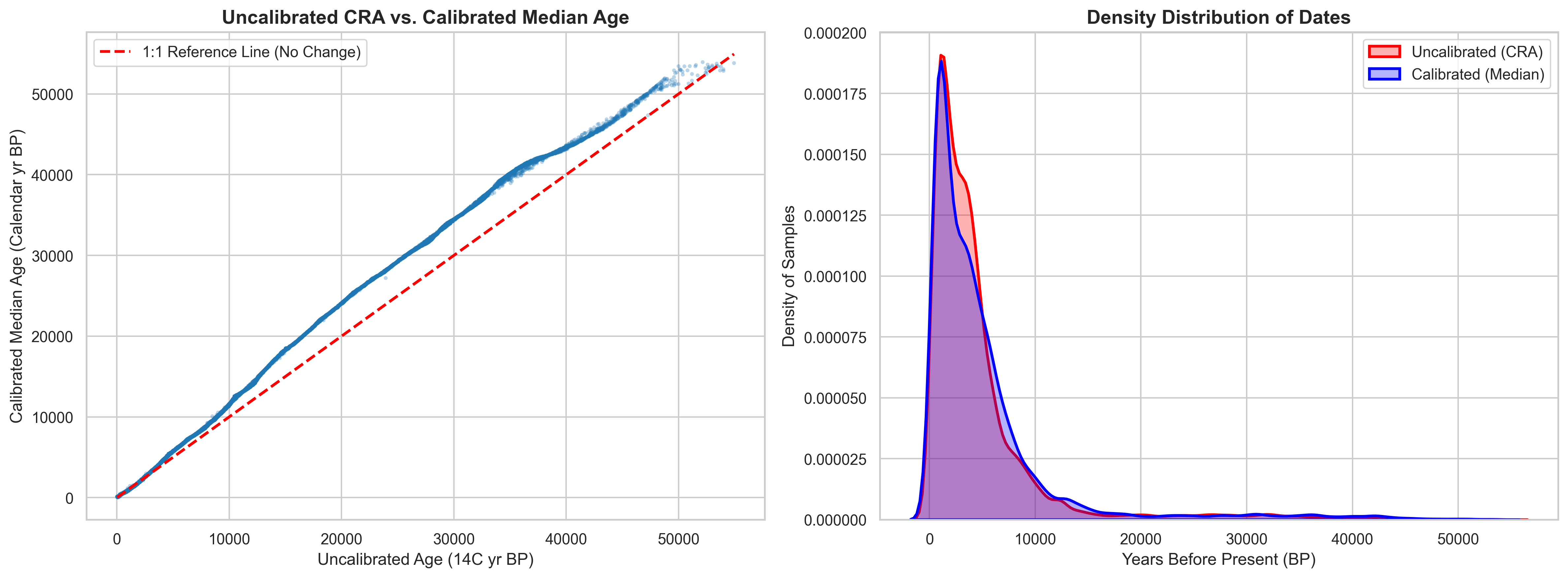
Radiocarbon ages must be calibrated via 02_Calibrating.py to account for historical fluctuations in atmospheric Carbon-14 (C14), especially during the Holocene.
Tools:
IOSACal (an open-source radiocarbon calibration library in Python) for Bayesian calibration, pandas for data management, and tqdm.
Functionality:
02_Calibrating.py automatically maps each date to the correct calibration curve (IntCal20 for the Northern Hemisphere, SHCal20 for the Southern Hemisphere) based on the sample's latitude. It extracts key numerical boundaries, such as the median calendar age and 95% confidence intervals, and formats them neatly into a pandas DataFrame for later analysis. This script outputs a p3k14c_pristine_dates.csv file, which will be used in the following statistical analyses.
- Curve selection: for every row, the script checks the "Lat" column. Any sample at or above the equator gets
intcal20; anything below getsshcal20. - Calibration: calls R(age, error, lab_id).calibrate(curve) from
IOSACalto get Cal BP data. - Extracting statistics: calls
.quantiles()on each CalAge result, which returns the median (quants[50]) and the 1σ / 2σ confidence intervals (quants[68], quants[95]).- 68.2% (1σ) confidence interval lower and upper bounds
- 95.4% (2σ) confidence interval lower and upper bounds
- Failure handling: rows with missing Age, Error, or Lat, or any row where
IOSACalthrows an exception, are written tocalibration_failures.csv.
Case Study: Çatalhöyük
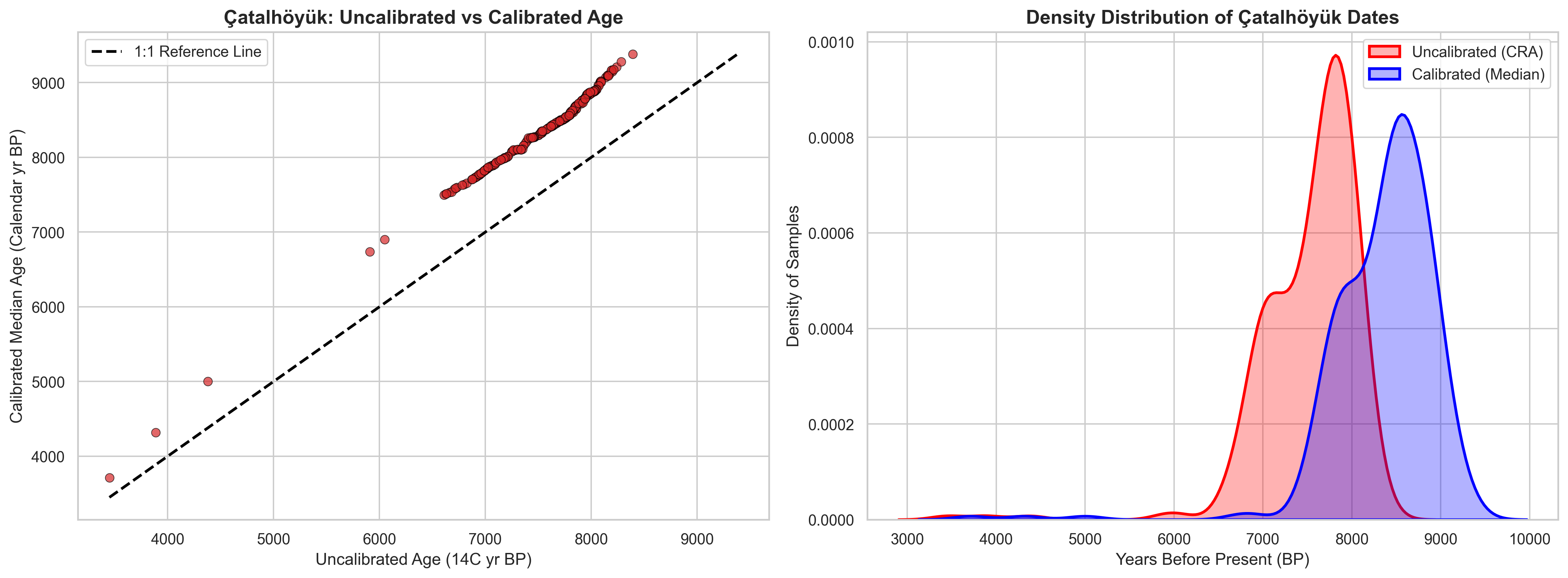
These Plots Show:
- Calibration Flattens and Spreads Time
- In Figures 2 & 3, the raw 14C ages (red) are naturally clustered and spiky due to plateaus in the calibration curve (where multiple calendar years produce the same radiocarbon age).
- Calibration (blue) smooths these spikes out, distributing the radiocarbon data accurately across the timeline.
- The "Hallstatt Plateau" Effect
- In Figure 3, note how the blue calibrated radiocarbon data is wider and lower than the red uncalibrated peak. This visually demonstrates why calibration is necessary: a single, precise radiocarbon measurement often corresponds to a broad range of true calendar years.
💡 Skip the setup! The final cleaned and calibrated dataset is in the GitHub repository (
Datasets/p3k14c_pristine_dates.csv). You can bypass the finicky cleaning and calibrating process entirely and jump straight to the data analysis.
Summary Statistics
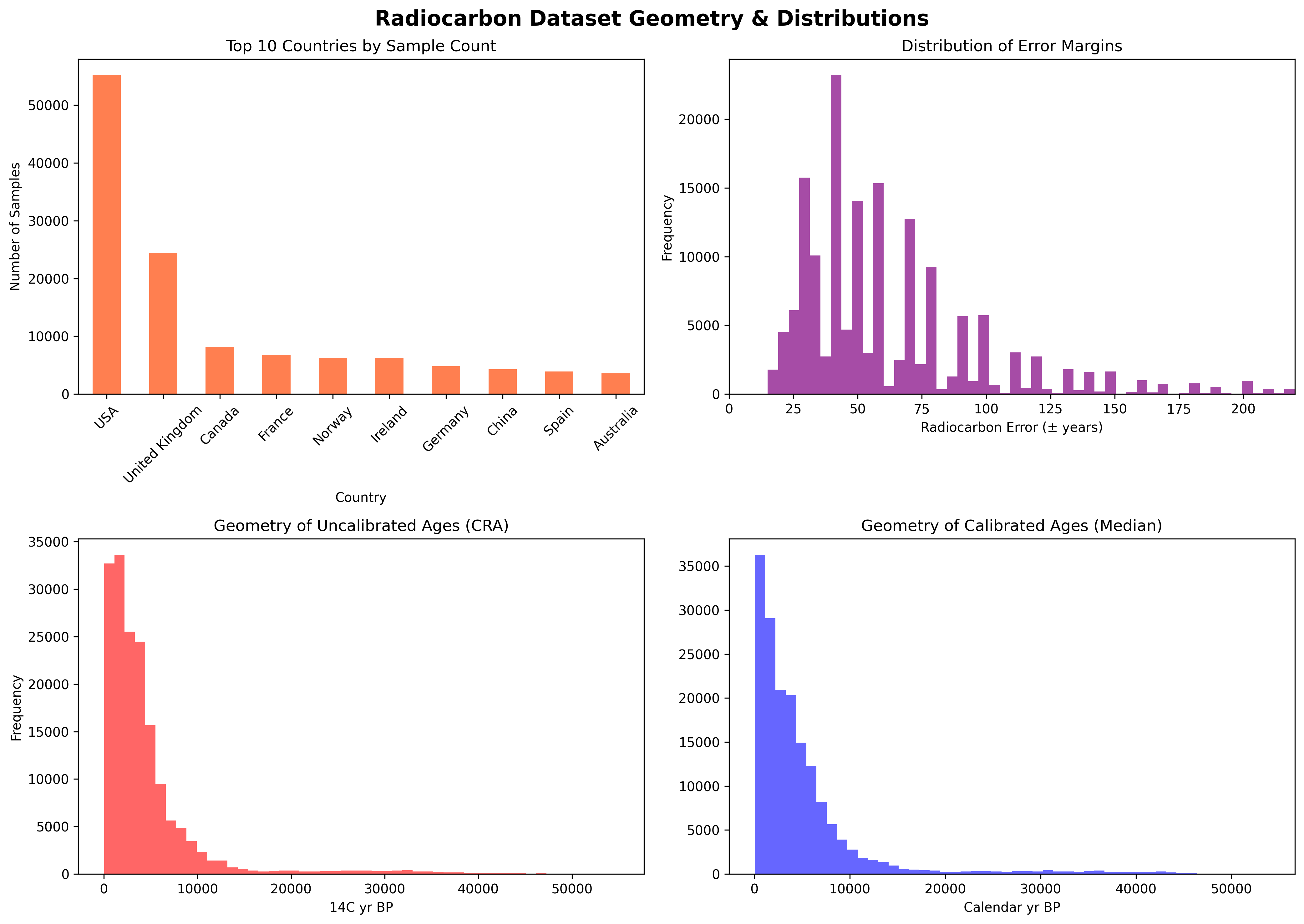
03_SummaryStats.py is a great first step to analyzing the large p3k14c dataset. Gives the researcher a general idea of the dataset's geometry and contents before diving into complex modeling.
Tools:
matplotlib.pyplot, pandas, and numpy.
Functionality:
03_SummaryStats.py generates summaries of continental and regional data, missing values, error margins, and distributions.
- Optional Country / SiteName filter (or press Enter for global view, shown below)
- Prints record counts, continental/country breakdowns, missing-value report, and age/error statistics (see below)
- Saves a 4-panel dashboard figure (see below)
 ========================================
        DATASET SUMMARY REPORT
========================================
Total Records: 169,051

--- Continental Breakdown ---
Continent
Europe           72082
North America    63388
Asia             13561
Africa            8960
South America     6253
Name: count, dtype: int64

--- Top 5 Countries ---
Country
USA               55213
United Kingdom    24414
Canada             8175
France             6805
Norway             6303
Name: count, dtype: int64

--- Missing Values ---
No missing values in key columns!

--- Age & Error Margins ---
                Count     Mean  Median   Min      Max
Age          169051.0  4540.92  3010.0  30.0  54940.0
Error        169051.0    89.86    55.0  15.0   9300.0
MedianCalBP  169051.0  5043.14  3191.0  48.0  53937.0
SPD (Summed Probability Distributions)
04_SPD.py can be used on calibrated radiocarbon data to estimate demographic fluctuations over time as a proxy for human activity. Essentially, the frequency of datable anthropogenic carbon recovered from archaeological contexts serves as a direct proxy for past fluctuations in human population density and associated settlement activity.
Tools:
scipy.optimize(differential_evolution, curve_fit) and scipy.stats(lineregress) for statistical modeling, radiocabon for age calibration, matplotlib, numpy, and pandas
Functionality:
04_SPD.py combines several methodologies from paleodemography:
- Chronometric Hygiene: Filters out problematic materials (old-wood/marine effects), drops large-error dates (Reimer et al. 2020).
- Spatial-Temoral Binning: Controls oversampling biases from single archaeological phases (Timpson et al. 2014).
- Taphonomic Correction: Applies power-function corrections to account for the natural decay and loss of organic material over time (Surovell et al. 2009; Bluhm & Surovell 2018).
- Null Hypothesis Significance Testing (NHST): Uses 5,000-iteration (adjustable) Monte Carlo simulations to test the empirical SPD against exponential and logistic null models, highlighting periods of statistically significant population deviation (Timpson et al. 2014; Crema et al. 2017; Weninger et al. 2015; Bettinger et al. 2016; Shennan et al. 2013).
- Continuous Piecewise Linear (CPL) Modelling: Uses differential evolution and Bayesian Information Criterion (BIC) to identify optimal "hinge points" that represent major regime shifts in population growth and decline (McLaughlin 2019; Edinborough et al. 2017).
Case Study: Çatalhöyük
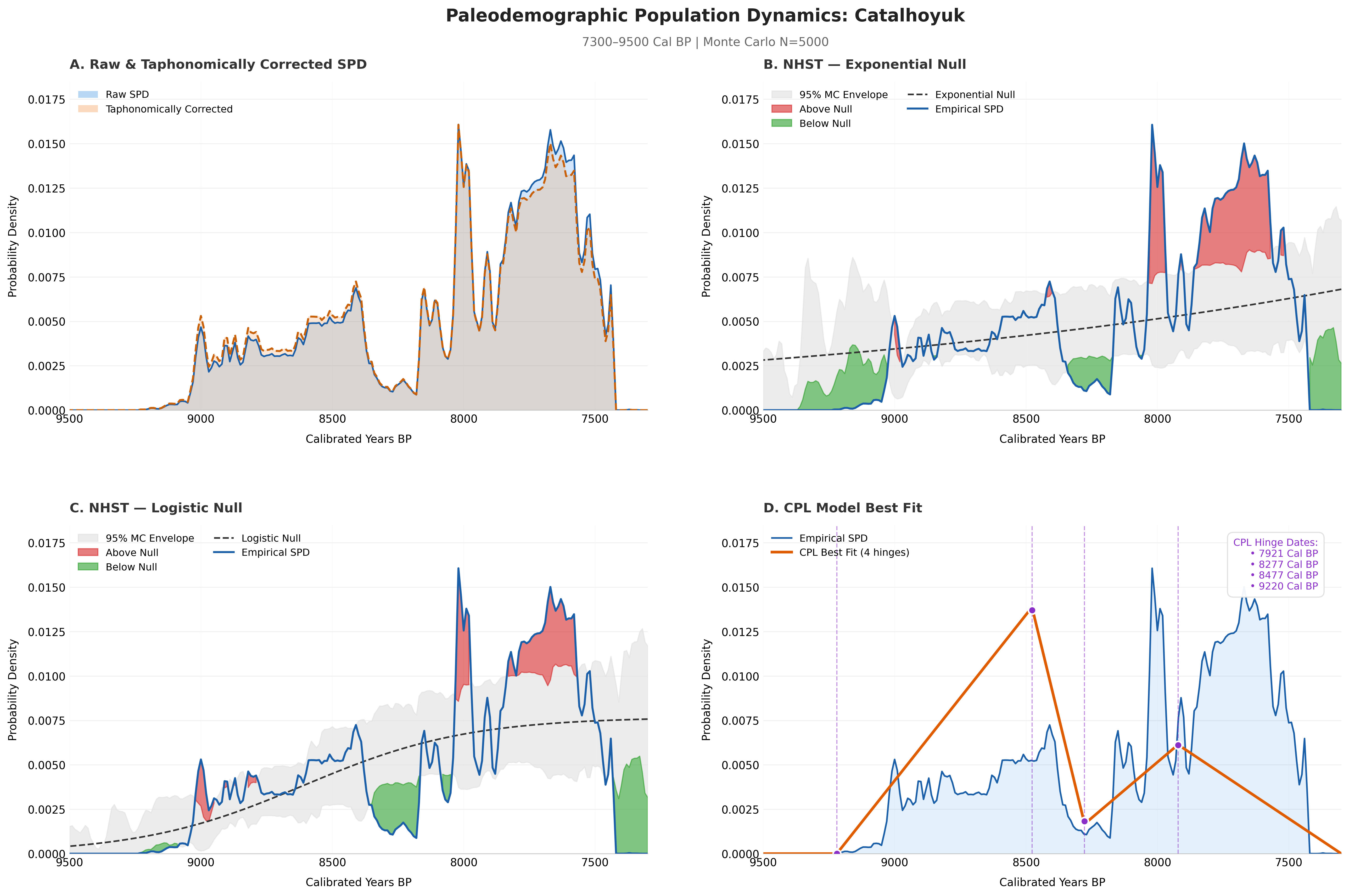
These Plots Show:
-
Initial Settlement and Growth (9220 - 8477 Cal BP)
- Plot D shows an initial hinge point at 9220 Cal BP, marking the beginning of an upward demographic trend
- Plots B & C show this growth tracking relatively closely with expected baselines, staying within the null envelope.
- Aligns with the settlement of the East mound.
-
Sudden Population Decline (8477 - 8277 Cal BP)
- Plot D shows a sharp drop at 8277 Cal BP, and Plots B & C show a red "Below Null" zone shortly after this period.
- This aligns with the 8.2 ky climate event and the "Late" phase, bringing about social fragmentation.
-
Population Boom (~8000 - 7500 Cal BP)
- Plot D shows a hinge point at 7921 Cal BP, showing a population recovery.
- Plot A spikes around this time.
- Plots B & C show massive red areas indicating "Above Null".
- This aligns with the occupation of the West mound; there may be sampling bias making this boom seem more prominent.
-
Final Decline (post 7500 Cal BP)
- Across all plots, a sharp decline is seen after 7500 Cal BP, marking the site's final abandonment.
Human - Environment Interactions
By merging the results from the SPD script with paleoclimate data, it can be elucidated whether or not a demographic trend was influenced by an environmental change. By overlaying the demographic proxy with smoothed environmental proxies, 05_Human_Climate_Interaction.py highlights distinct periods of environmental stress and then evaluates whether corresponding demographic drops (identified via Monte Carlo significance testing) represent true societal collapses and/or recoveries.
Tools:
requests for querying web APIs, scipy.interpolate(interp1d) for time-series alignment, scipy.signal(savgol_filter, detrend) for smoothing, and matplotlib/seaborn.
Functionality:
- Automated Data Retrieval: Fetches local environmental proxy data (e.g., stable isotopes, pollen) from PANGAEA and Neotoma databases based on proximity to the archaeological site.
- Data Harmonization: Detrends and Z-scores disparate environmental proxies, aligning them temporally with the IntCal20-calibrated demographic SPD.
- Anomaly Detection: Identifies periods of extreme environmental stress (anomalies) using customizable thresholds.
- Resilience & Resistance Metrics: Calculates the demographic resistance to an environmental event, and fits an exponential recovery curve to quantify subsequent human resilience.
- Visualization: Generates a comprehensive, multi-panel dashboard comparing demographic and environmental Z-scores over time.
Case Study: Çatalhöyük
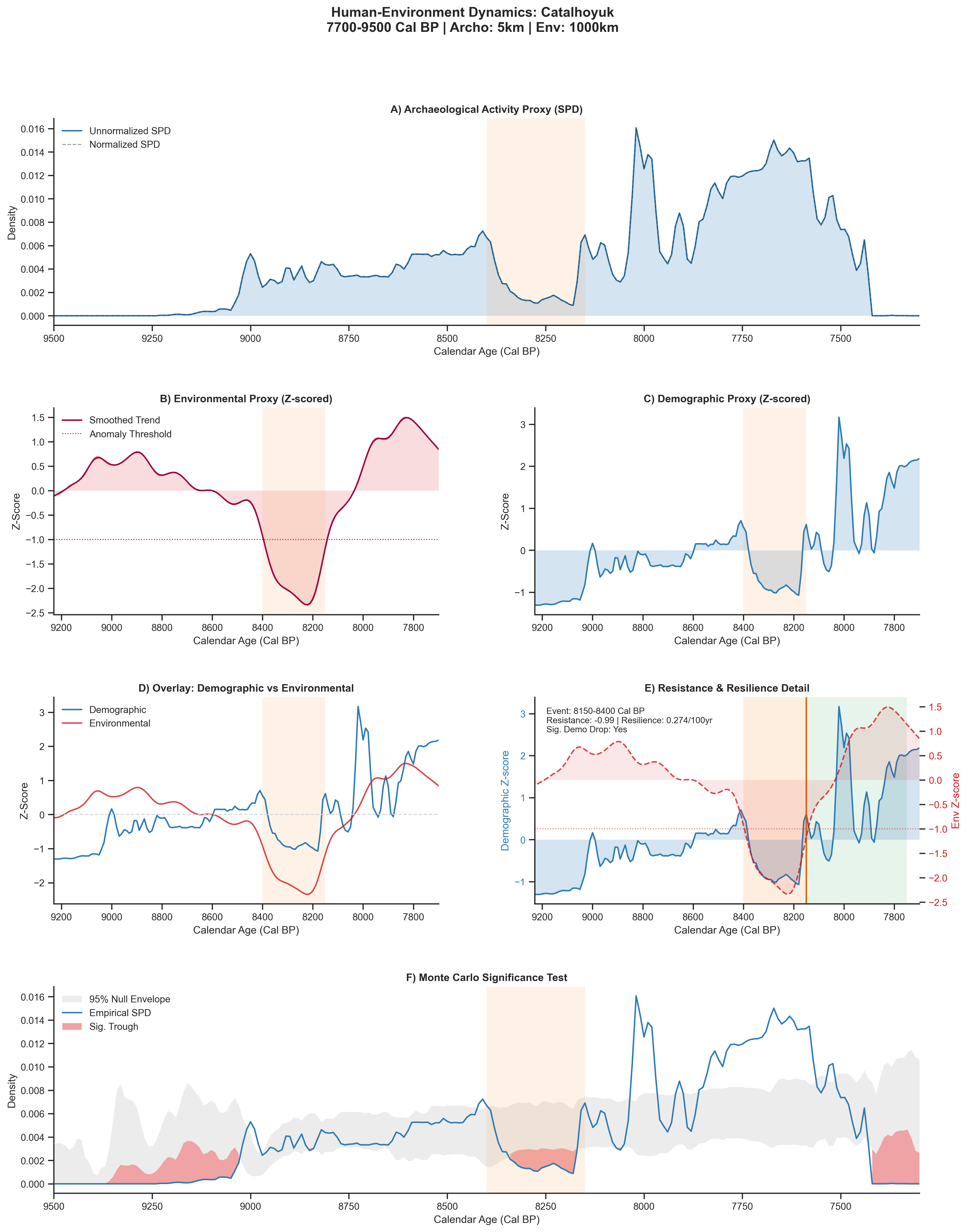
These Plots Show:
-
Environmental Shock (8400 - 8150 Cal BP)
- The Environmental Proxy Plot (B) shows a sharp decline in the environmental Z-score reaching well below the -1.0 anomaly threshold
- This aligns well with the 8.2 ky event (abrupt global cooling and aridification)
-
Human - Environment Interaction
- The Archaeological Activity Proxy Plot (A) and the Demographic Proxy Plot (C) both exhibit a sharp decline in synch with the environmental change.
- The Resistance & Resilience Detail Pot (E) and the Monte Carlo Significance Test (F) confirm that this was not a random fluctuation, meaning the climate event forced a genuine demographic change.
-
Shock Aftermath (~8000 - 7500 Cal BP)
- The Overlay Plot (D) shows that as soon as the climate recovers, the population follows almost immediately.
- By 8000 Cal BP, the archaeological activity surpasses the previous levels, exhibiting high societal resilience (noted as 0.274/100yr in the detail plot).
- This shows that the population at Çatalhöyük adapted, reorganized, and recovered once the climate stabilized.
- From the Ice Core data, it is unclear whether the final abandonment of the site was climate-motivated.
Composite Paleoproxies for Human - Environment Interactions
To create a more robust understanding of past climate stressors, it is often helpful to synthesize multiple lines of environmental evidence. Relying on a single proxy can introduce regional bias or data gaps. 06_Composite_Human_Environment.py uses Principal Component Analysis (PCA) to distill multiple paleoclimate datasets (e.g., ice core temperatures, pollen counts, and stable isotopes) into a single, comprehensive Composite Climate Stress Index (CCSI).
Tools:
sklearn.decomposition(PCA), sklearn.preprocessing(StandardScaler), scipy, and pandas.
Functionality:
- Fetches multiple palaeoclimate proxy series for the specified site from:
- NOAA GISP2 —> Greenland temperature (global signal, always available)
- PANGAEA —> any keyword-matched proxies (e.g. speleothem d18O)
- Neotoma —> pollen-based proxies (precipitation/vegetation)
- Bins every proxy to the same temporal grid (RESOLUTION yr steps).
- Z-scores each proxy individually (so units are commensurable).
- Applies PCA across proxies; PC1 is retained as the Composite Climate Stress Index (CCSI).
- Sign convention: positive CCSI = warm/wet, negative = cold/dry/stressed.
- If the leading PC points the "wrong way," it is automatically flipped so that lower values always = more climate stress.
- Compares CCSI against the demographic SPD (loaded from 04's output or rebuilt from scratch).
- Detects climate stress episodes (CCSI < threshold), calculates resistance and resilience exactly as in 06_Human_Environment.py.
- Saves files:
- _ccsi.csv — gridded CCSI + each proxy Z-score
- _ccsi_resilience.csv — per-episode resistance/resilience table
- _ccsi.png — 5-plot figure (see below)
Case Study: Çatalhöyük
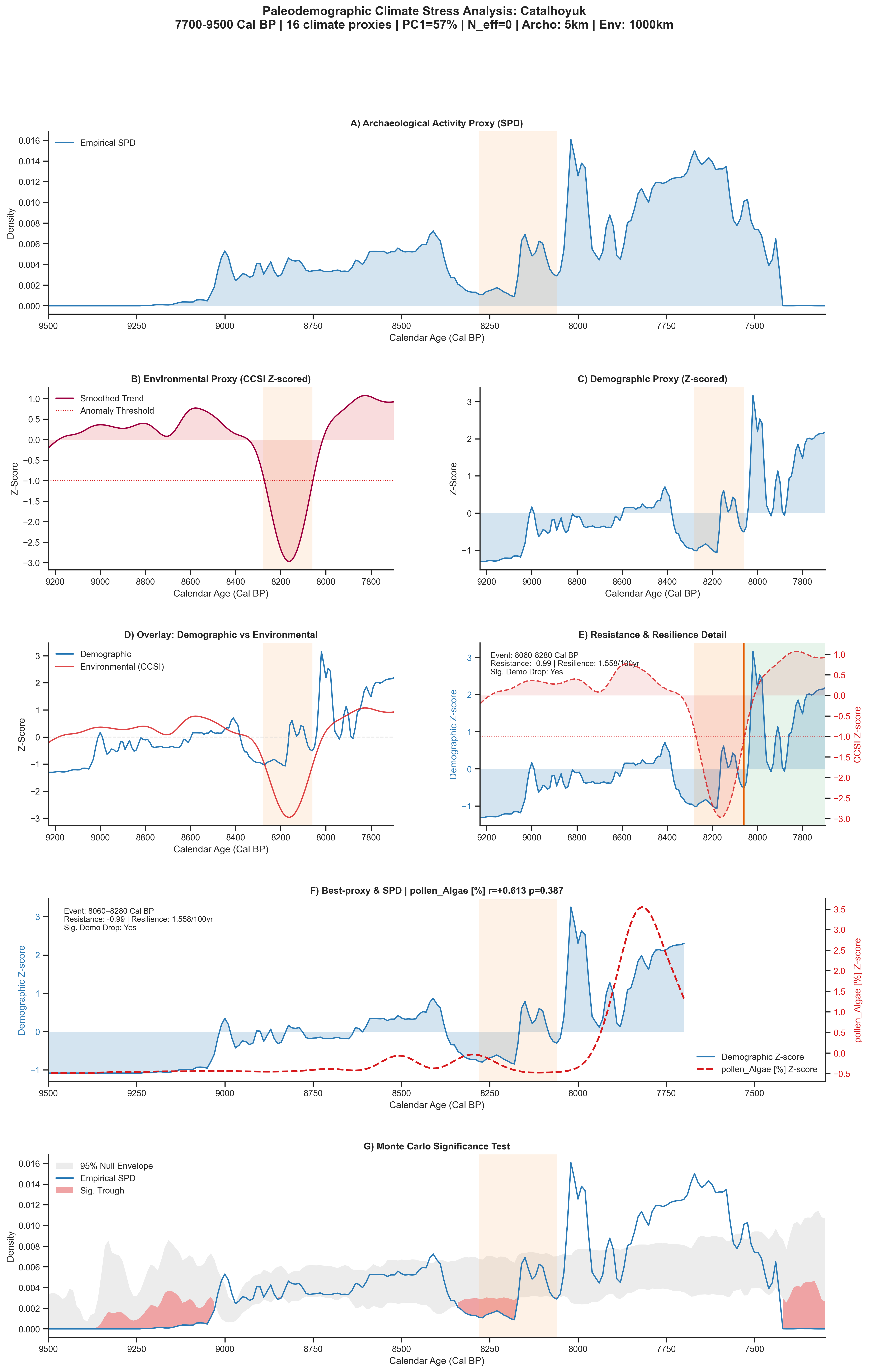
These Plots Show:
-
Environmental Shock (8280 - 8000 Cal BP)
- The Environmental CCSI Plot (B) shows a sharp decline in the environmental Z-score reaching well below the -1.0 anomaly threshold
- This aligns perfectly with the 8.2 ky event (abrupt global cooling and aridification)
-
Difference between Fig. 6 & 7
- By this model, the anomaly period is slightly later and sharper, spanning ~8280 - 8000 Cal BP, when concerning the pollen data.
- The population is shown to have already been crashing when the 8.2-kiloyear climate event hit.
- This could be due to ecological lag and/or calibration error.
Density Analysis
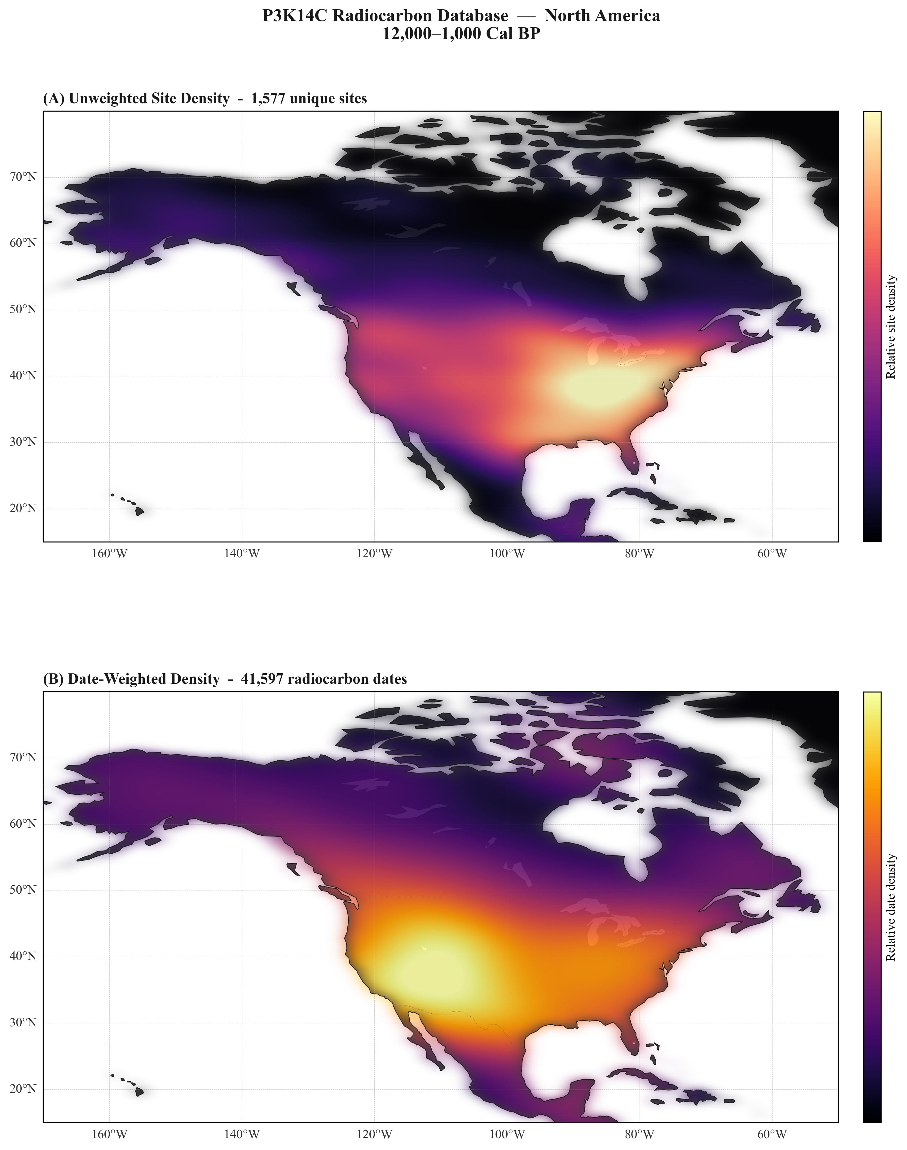
07_KDE.py shows the geographical distribution of unweighted sites across a region (A) and the weighted C14 dates at those sites (B). This script allows the user to select a specific temporal range and region (one of the seven continents) or create a custom region (via latitude and longitude) for analysis.
Tools:
cartopy(ccrs, cfeature) for map projections and geography, scipy.stats(gaussian_kde) for density estimation, and matplotlib.
Functionality:
07_KDE.py uses scipy.stats.gaussian_kde to create continuous Kernel Density Estimation (KDE) surfaces for recorded sites vs. dated sites as follows:
- Prompts for a geographic region (preset or custom bounding box)
- Prompts for a temporal window (Cal BP)
- Computes two KDE surfaces:
- (A) Unweighted — each unique site location counts equally
- (B) Date-weighted — sites with more 14C dates contribute more
- Saves a 2-panel map figure (PNG) masked to land
1 maintainer

Metadata
1 maintainer
Release files for paleopy 0.1.0
For a detailed explanation of source distributions (sdists) and built distributions (wheels), please see the package formats documentation.
Source distribution (sdist)
| File | Size | Uploaded | |
|---|---|---|---|
| paleopy-0.1.0.tar.gz | 94.0 kB | Details |
Built distribution (wheel)
| File | Interpreter | ABI | Platform | Reset |
|---|---|---|---|---|
| paleopy-0.1.0-py3-none-any.whl | Python 3 | none | any | Details |
Total release size: 175.5 kB
Release files / paleopy-0.1.0.tar.gz
| Download URL | paleopy-0.1.0.tar.gz |
|---|---|
| Size | 94.0 kB |
| Tags | Source |
|
SHA-256 checksum How to use checksums |
59da1c723b33aa126bb3c4793974ed117c5578d3b4d8c7872a1de697b8c62e01
|
|
BLAKE2b-256 checksum How to use checksums |
6dd7bb9f71557098419020dd3d2d43141f76b3940abbfe883baef2a3e4dc73e3
|
| Upload date | |
|
Uploaded using Trusted Publishing? What is trusted publishing? |
No |
| Uploaded via |
twine/7.0.0 CPython/3.12.10
|
Release files / paleopy-0.1.0-py3-none-any.whl
| Download URL | paleopy-0.1.0-py3-none-any.whl |
|---|---|
| Size | 81.5 kB |
| Tags | Python 3 |
|
SHA-256 checksum How to use checksums |
409db68fd02b2785bb503e8ed93011cc3239cc1544f40cab6366dae5ca3299ee
|
|
BLAKE2b-256 checksum How to use checksums |
fc627879352527484347b44b71fe521fc4ffaf98374d8016d61bc3a031a84be9
|
| Upload date | |
|
Uploaded using Trusted Publishing? What is trusted publishing? |
No |
| Uploaded via |
twine/7.0.0 CPython/3.12.10
|













