
panelmed


panelmed implements the double/debiased machine learning estimator for causal mediation analysis in panel data of Wu and Xiao (2026), arXiv:2610.21339, in Python. You give it a panel with an outcome, a mediator, a treatment and covariates; it returns the direct, indirect and total effects of the treatment with standard errors, tables ready for a manuscript, and figures.
- Documentation: https://merwanroudane.github.io/panelmed/
- PyPI: https://pypi.org/project/panelmed/
- Author: Dr Merwan Roudane · merwanroudane920@gmail.com · https://github.com/merwanroudane
Table of contents
- What this package does
- Start from absolutely nothing
- Installation
- Your first analysis in 60 seconds
- Complete example with real data
- Full syntax reference
- Interpreting the output
- Using your own Excel or CSV file
- Exporting tables and figures
- The method
- Practical guidance and pitfalls
- Limitations
- References
- Citation
- Author and licence
1. What this package does
Many questions ask not only whether a treatment changes an outcome but through which channel. Employment raises local income: how much of that goes through wages? Mediation analysis splits the total effect into a direct effect and an indirect effect that passes through a mediator. With panel data the difficulty is that unobserved, time-invariant characteristics of each unit can drive treatment, mediator and outcome at once, and that observed confounders may act nonlinearly.
The estimator of Wu and Xiao (2026) handles both. It allows unit and period fixed effects in all three equations, lets unknown nonlinear functions of the covariates absorb observed confounding, and uses cross-fitting so that the machine-learning step does not bias the estimates.
What you get:
- Estimator: DML-GMM for the outcome and mediator equations (Algorithm 1 of the paper).
- Effects: controlled direct, natural direct, natural indirect and total effects, as level contrasts between two treatment histories and as derivatives.
- Inference: analytical standard errors from influence functions, joint Wald tests, and a cross-sectional bootstrap that repeats the whole procedure.
- Comparisons: the naive benchmark of the paper, and a paired test of whether two specifications give different decompositions.
- Beyond the paper: two-step GMM with the Hansen J test, an analytical standard error for the mediated share, and a moment-diagnostic figure.
- Output: text, LaTeX, Markdown and HTML tables; six figure types.
- Data: the U.S. county panel used in the paper's application, and the paper's Monte Carlo generator.
2. Start from absolutely nothing
If you have never used Python, do these four steps once. Fifteen minutes.
Step 1 - install Python
Download Anaconda (recommended for researchers: it includes Python, Jupyter and Spyder in one installer) from https://www.anaconda.com/download, or plain Python from https://www.python.org/downloads/. On the python.org installer, tick "Add Python to PATH" on the first screen.
Step 2 - open a terminal
- Windows: press
Win, typeAnaconda Prompt(orcmd), press Enter. - macOS: press
Cmd+Space, typeTerminal, press Enter.
Check it works. Type this and press Enter:
python --version
You should see something like Python 3.11.5.
Step 3 - install this package
pip install panelmed
Step 4 - run your first command
Type python, press Enter, then paste:
import panelmed
print(panelmed.__version__)
Type exit() to leave.
Where do I write my code?
Any of these; pick one and stay with it.
| Tool | Best for | How to open |
|---|---|---|
| Jupyter Notebook | step-by-step work with figures inline | type jupyter notebook in the terminal |
| Spyder | a MATLAB/RStudio-like window | type spyder, or open it from Anaconda Navigator |
A .py file |
a reproducible script | save analysis.py, then run python analysis.py |
3. Installation
pip install panelmed
With interactive 3-D surfaces:
pip install "panelmed[plotly]"
Development version:
pip install git+https://github.com/merwanroudane/panelmed.git
Requirements: Python >= 3.10, numpy, scipy, pandas, matplotlib, scikit-learn, joblib (installed automatically).
4. Your first analysis in 60 seconds
from panelmed import PanelMediation, simulate_panel

# a simulated panel with known true effects: 1,600 units, 10 periods
df = simulate_panel(n=1600, t=10, seed=2026, as_frame=True)

model = PanelMediation(
    "y", "m", "d", ["x1", "x2", "x3", "x4", "x5"],      # outcome, mediator, treatment, covariates
    data=df, unit="unit", time="time",
    outcome=["d", "d**2", "L1_d", "d*x3", "m", "L1_m"],  # what enters the outcome equation
    mediator=["d", "d**2", "L1_d"],                      # what enters the mediator equation
)
res = model.fit(n_folds=10, seed=2026)
print(res.effects(d=1, d_star=0).summary())
======================================================================================
                  Panel mediation, level effects  (Wu & Xiao (2026))
======================================================================================
Outcome            : y                                 Units (N)        :         1600
Mediator           : m                                 Periods (T)      :           10
Treatment          : d                                 Folds (K)        :           10
Covariates         : 5                                 Instrument lags  :            2
Basis              : polynomial deg. 3 (55 terms)      Moments          :           83
Estimator          : DML-GMM                           Weighting        :     identity
--------------------------------------------------------------------------------------
Estimand        Coef.  Std.Err.        z   P>|z|      [95% Conf. Int.]
--------------------------------------------------------------------------------------
Effects
CDE            4.5065    0.0737   61.184   0.000     4.3621     4.6508 ***
NDE            4.5065    0.0737   61.184   0.000     4.3621     4.6508 ***
NIE            2.7899    0.0942   29.630   0.000     2.6053     2.9744 ***
TE             7.2964    0.1072   68.033   0.000     7.0862     7.5066 ***
--------------------------------------------------------------------------------------
Mediated share
NIE/TE         0.3824    0.0095                      0.3637     0.4010
======================================================================================
Significance: *** p<0.01, ** p<0.05, * p<0.10
Standard errors: estimated influence functions (Eq. 21, Theorem 3).
Treatment history d versus d*; mediator fixed at m for the CDE.
Total = natural direct + natural indirect. No test against zero is reported for the mediated share.
The true values in this simulated design are CDE = NDE = 4.5, NIE = 3 and TE = 7.5.
5. Complete example with real data
The package ships the panel used in the empirical application of Wu and Xiao (2026, Section 6): 3,058 U.S. counties observed every year from 2000 to 2019, assembled by Cerqua, Letta and Pinto (2026). The question: when the workplace employment rate of a county rises, personal income per capita rises too. How much of that goes through the average wage?
| Role | Variable | Definition |
|---|---|---|
Outcome y |
log personal income per capita | USD, in logs |
Mediator m |
log average wage per job | USD, in logs |
Treatment d |
workplace employment rate | jobs located in the county per resident aged 18-65 |
| Covariates | 8 county characteristics, measured the year before | log population, share of income from unemployment insurance, population shares under 18 and over 65, births, deaths, net international and net domestic migration per 1,000 residents |
load_us_counties() returns the panel prepared as in the paper: years 2001-2019
(the year 2000 only supplies the lagged covariates), every variable winsorised at its
1% and 99% quantiles and standardised. Effects are therefore in standard deviations
of the outcome per standard deviation of the treatment.
The whole example is the script
examples/panelmed_empirical.py; the output below
is copied from a run of that script.
Step 1 - load the data
from panelmed import PanelMediation, compare_effects, load_us_counties
from panelmed.datasets import US_COUNTIES_COVARIATES as X

df = load_us_counties()
print(df.head(3).round(3).to_string(index=False))
 county_id        county_name  year      y      m      d  log_pop  ui_share  share_under18  share_over65  births  deaths  mig_international  mig_domestic
      1001 Autauga County, AL  2001 -1.054 -1.189 -0.929    0.297    -0.769          1.507        -1.392  -2.104  -2.174             -0.581         0.353
      1001 Autauga County, AL  2002 -0.991 -1.079 -1.036    0.310    -0.636          1.425        -1.368   0.798  -0.457             -0.568         0.714
      1001 Autauga County, AL  2003 -0.795 -1.029 -1.013    0.326    -0.450          1.473        -1.346   0.471  -0.427             -0.960         1.156

Counties: 3058, years: 2001-2019
Step 2 - Specification I: the same effect in every county
common = dict(data=df, unit="county_id", time="year", basis_degree=3, basis_max_vars=2)

spec1 = PanelMediation("y", "m", "d", X, outcome=["d", "m"], mediator=["d"], **common)
res1 = spec1.fit(n_folds=5, max_lags=2, seed=2026)
print(res1.summary())
======================================================================================
              Panel mediation, structural parameters  (Wu & Xiao (2026))
======================================================================================
Outcome            : y                                 Units (N)        :         3058
Mediator           : m                                 Periods (T)      :           19
Treatment          : d                                 Folds (K)        :            5
Covariates         : 8                                 Instrument lags  :            2
Basis              : polynomial deg. 3 (108 terms)     Moments          :           99
Estimator          : DML-GMM                           Weighting        :     identity
--------------------------------------------------------------------------------------
Parameter       Coef.  Std.Err.        z   P>|z|      [95% Conf. Int.]
--------------------------------------------------------------------------------------
Outcome equation (theta)
theta[d]       0.2089    0.0875    2.388   0.017     0.0375     0.3803 **
theta[m]       0.6593    0.0943    6.991   0.000     0.4744     0.8441 ***
--------------------------------------------------------------------------------------
Mediator equation (gamma)
gamma[d]       0.6063    0.0780    7.775   0.000     0.4535     0.7592 ***
======================================================================================
Significance: *** p<0.01, ** p<0.05, * p<0.10
Sandwich standard errors from the stacked individual scores (Eq. A.15); N -> infinity, T fixed.
Moments: 66 outcome + 33 mediator; Jacobian condition number 2.0.
Step 3 - Specification II: effects that vary with county characteristics
inter = [f"d*{c}" for c in X]          # d*log_pop, d*ui_share, ...
spec2 = PanelMediation("y", "m", "d", X, outcome=["d", "m"] + inter,
                       mediator=["d"] + inter, **common)
res2 = spec2.fit(n_folds=5, max_lags=2, seed=2026)
print(res2.summary())
==================================================================================================
                    Panel mediation, structural parameters  (Wu & Xiao (2026))
==================================================================================================
Outcome            : y                                             Units (N)        :         3058
Mediator           : m                                             Periods (T)      :           19
Treatment          : d                                             Folds (K)        :            5
Covariates         : 8                                             Instrument lags  :            2
Basis              : polynomial deg. 3 (108 terms)                 Moments          :          627
Estimator          : DML-GMM                                       Weighting        :     identity
--------------------------------------------------------------------------------------------------
Parameter                       Coef.  Std.Err.        z   P>|z|      [95% Conf. Int.]
--------------------------------------------------------------------------------------------------
Outcome equation (theta)
theta[d]                       0.3657    0.1176    3.109   0.002     0.1352     0.5962 ***
theta[m]                       0.5264    0.1110    4.743   0.000     0.3088     0.7439 ***
theta[d*log_pop]              -0.0058    0.0613   -0.095   0.924    -0.1259     0.1142
theta[d*ui_share]              0.0045    0.0102    0.439   0.661    -0.0155     0.0245
theta[d*share_under18]         0.1907    0.0748    2.550   0.011     0.0441     0.3373 **
theta[d*share_over65]          0.2314    0.0648    3.571   0.000     0.1044     0.3583 ***
theta[d*births]               -0.0206    0.0110   -1.873   0.061    -0.0421     0.0010 *
theta[d*deaths]                0.0089    0.0132    0.669   0.503    -0.0171     0.0348
theta[d*mig_international]     0.0344    0.0116    2.966   0.003     0.0117     0.0572 ***
theta[d*mig_domestic]         -0.0055    0.0079   -0.698   0.485    -0.0210     0.0100
--------------------------------------------------------------------------------------------------
Mediator equation (gamma)
gamma[d]                       0.4715    0.0905    5.210   0.000     0.2942     0.6489 ***
gamma[d*log_pop]              -0.0247    0.0560   -0.440   0.660    -0.1345     0.0851
gamma[d*ui_share]             -0.0217    0.0074   -2.923   0.003    -0.0362    -0.0071 ***
gamma[d*share_under18]        -0.0331    0.0279   -1.189   0.234    -0.0877     0.0215
gamma[d*share_over65]         -0.0038    0.0346   -0.109   0.913    -0.0715     0.0640
gamma[d*births]               -0.0083    0.0067   -1.232   0.218    -0.0214     0.0049
gamma[d*deaths]                0.0125    0.0092    1.359   0.174    -0.0055     0.0306
gamma[d*mig_international]     0.0006    0.0062    0.102   0.919    -0.0115     0.0127
gamma[d*mig_domestic]         -0.0012    0.0054   -0.222   0.824    -0.0118     0.0094
==================================================================================================
Significance: *** p<0.01, ** p<0.05, * p<0.10
Sandwich standard errors from the stacked individual scores (Eq. A.15); N -> infinity, T fixed.
Moments: 330 outcome + 297 mediator; Jacobian condition number 23.6.
Step 4 - direct, indirect and total effects, averaged over 2001-2019
eff1 = res1.derivatives(d=0, period="average")
eff2 = res2.derivatives(d=0, period="average")
print(eff1.summary())
print(eff2.summary())
======================================================================================
               Panel mediation, derivative effects  (Wu & Xiao (2026))
======================================================================================
Outcome            : y                                 Units (N)        :         3058
Mediator           : m                                 Periods (T)      :           19
Treatment          : d                                 Folds (K)        :            5
Covariates         : 8                                 Instrument lags  :            2
Basis              : polynomial deg. 3 (108 terms)     Moments          :           99
Estimator          : DML-GMM                           Weighting        :     identity
--------------------------------------------------------------------------------------
Estimand        Coef.  Std.Err.        z   P>|z|      [95% Conf. Int.]
--------------------------------------------------------------------------------------
Effects
CDD            0.2089    0.0875    2.388   0.017     0.0375     0.3803 **
NDD            0.2089    0.0875    2.388   0.017     0.0375     0.3803 **
NID            0.3997    0.0703    5.689   0.000     0.2620     0.5375 ***
TD             0.6086    0.0786    7.746   0.000     0.4546     0.7626 ***
--------------------------------------------------------------------------------------
Mediated share
NID/TD         0.6568    0.1199                      0.4218     0.8918
======================================================================================
Significance: *** p<0.01, ** p<0.05, * p<0.10
Standard errors: estimated influence functions (Eq. 21, Theorem 3).
Derivative with respect to the treatment of the effect's own period.
Total = natural direct + natural indirect. No test against zero is reported for the mediated share.
======================================================================================
               Panel mediation, derivative effects  (Wu & Xiao (2026))
======================================================================================
Outcome            : y                                 Units (N)        :         3058
Mediator           : m                                 Periods (T)      :           19
Treatment          : d                                 Folds (K)        :            5
Covariates         : 8                                 Instrument lags  :            2
Basis              : polynomial deg. 3 (108 terms)     Moments          :          627
Estimator          : DML-GMM                           Weighting        :     identity
--------------------------------------------------------------------------------------
Estimand        Coef.  Std.Err.        z   P>|z|      [95% Conf. Int.]
--------------------------------------------------------------------------------------
Effects
CDD            0.3657    0.1177    3.107   0.002     0.1350     0.5964 ***
NDD            0.3657    0.1177    3.107   0.002     0.1350     0.5964 ***
NID            0.2482    0.0478    5.193   0.000     0.1545     0.3419 ***
TD             0.6139    0.1051    5.843   0.000     0.4080     0.8198 ***
--------------------------------------------------------------------------------------
Mediated share
NID/TD         0.4043    0.1068                      0.1949     0.6137
======================================================================================
Significance: *** p<0.01, ** p<0.05, * p<0.10
Standard errors: estimated influence functions (Eq. 21, Theorem 3).
Derivative with respect to the treatment of the effect's own period.
Total = natural direct + natural indirect. No test against zero is reported for the mediated share.
Compared with Table 2 of the paper:
| NDD | NID | TD | NID/TD | |
|---|---|---|---|---|
| Specification I, paper | 0.2145 | 0.4017 | 0.6162 | 0.6519 |
| Specification I, panelmed | 0.2089 | 0.3997 | 0.6086 | 0.6568 |
| Specification II, paper | 0.3597 | 0.2502 | 0.6099 | 0.4103 |
| Specification II, panelmed | 0.3657 | 0.2482 | 0.6139 | 0.4043 |
The small differences come from the random fold split, which the paper does not
publish. The paper reports bootstrap standard errors (500 replications); the tables
above use the analytical ones. For bootstrap standard errors run
python panelmed_empirical.py 200 (slow: every replication repeats the whole
procedure).
Step 5 - does the decomposition change between the two specifications?
print(compare_effects(eff1, eff2))
======================================================================================
         Paired difference between specifications (B - A)  (Wu & Xiao (2026))
======================================================================================
Outcome            : y                                 Units (N)        :         3058
Mediator           : m                                 Periods (T)      :           19
Treatment          : d                                 Folds (K)        :            5
Covariates         : 8                                 Instrument lags  :            2
Basis              : polynomial deg. 3 (108 terms)     Moments          :          627
Estimator          : DML-GMM                           Weighting        :     identity
--------------------------------------------------------------------------------------
Estimand        Coef.  Std.Err.        z   P>|z|      [95% Conf. Int.]
--------------------------------------------------------------------------------------
CDD            0.1568    0.0762    2.056   0.040     0.0074     0.3062 **
NDD            0.1568    0.0762    2.056   0.040     0.0074     0.3062 **
NID           -0.1515    0.0510   -2.972   0.003    -0.2515    -0.0516 ***
TD             0.0053    0.0698    0.075   0.940    -0.1315     0.1421
NID/TD        -0.2525    0.0813   -3.105   0.002    -0.4119    -0.0931 ***
======================================================================================
Significance: *** p<0.01, ** p<0.05, * p<0.10
Standard errors: difference of the unit-level influence functions.
The total effect is the same in both specifications, but the share going through wages drops from about two thirds to about 40%. This is the paper's main empirical message: a stable total effect does not validate its direct/indirect split.
Step 6 - figures
fig, ax = eff2.plot()
fig.savefig("decomposition.pdf")
res2.derivatives(d=0, period="all").plot_profile()
res2.plot_dose_response()
res2.plot_surface()
res1.plot_moments()
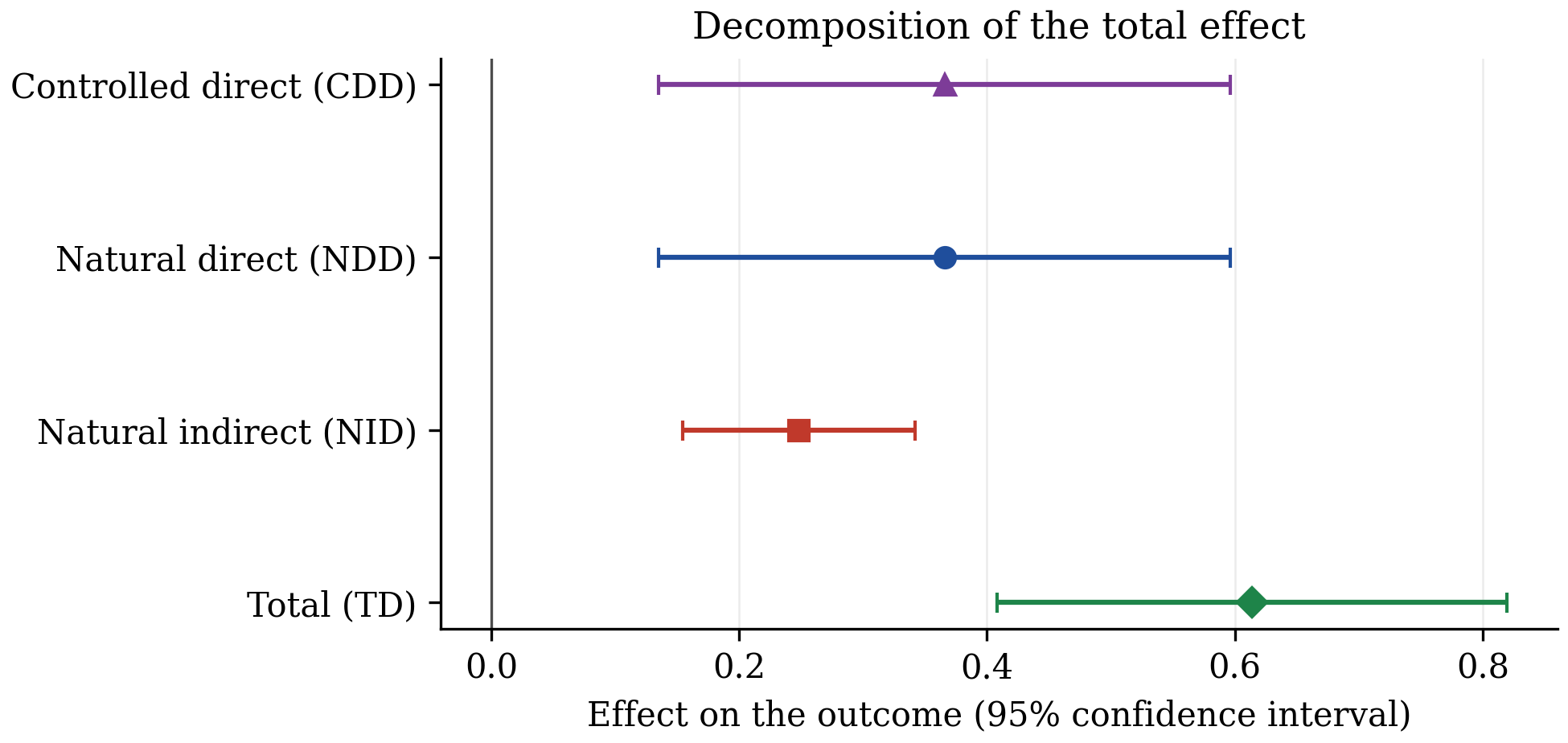
Direct, indirect and total effect under Specification II, with 95% intervals.
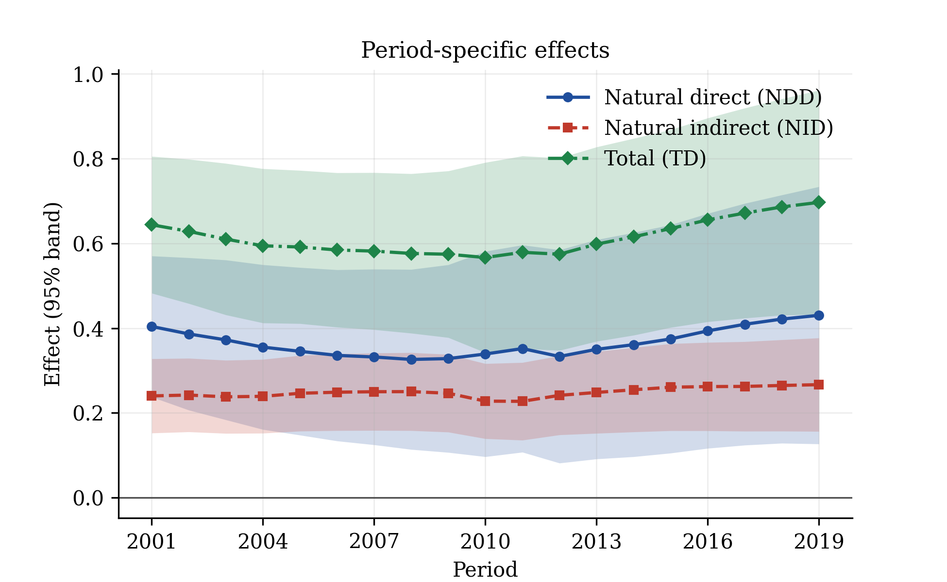
Year-by-year effects under Specification II. All three profiles are mildly U-shaped, as in Figure A.1 of the paper.
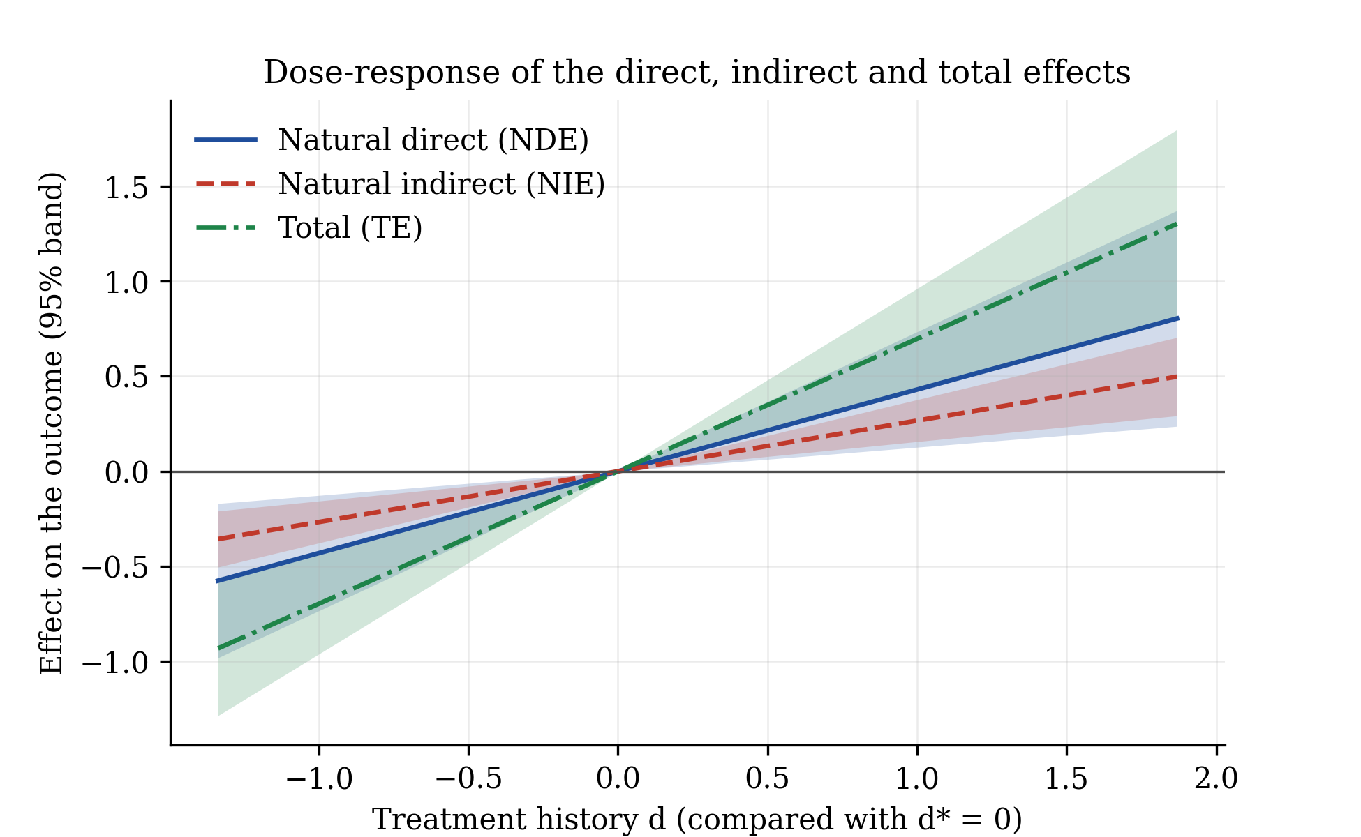
Effects of moving the employment rate from 0 (its mean) to each value d, in
standard deviations.
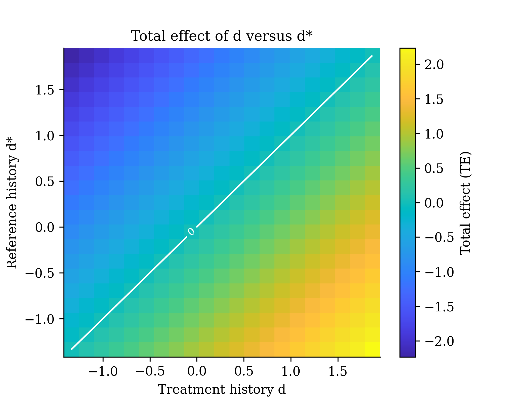
Total effect for every pair of treatment histories (d, d*).
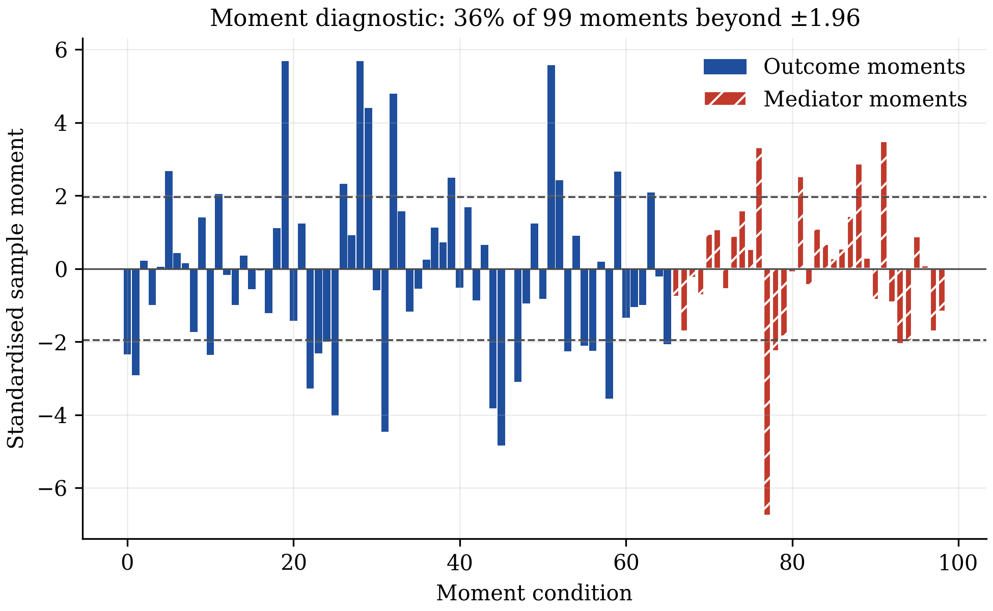
Standardised sample moments of Specification I at the estimate.
6. Full syntax reference
PanelMediation(y, m, d, x=None, *, outcome, mediator, ...)
Sets up the model of Eq. (4) of the paper.
| Argument | Type | Default | Meaning |
|---|---|---|---|
y, m, d |
column names, or (N, T) arrays |
required | outcome, continuous mediator, treatment (binary, multivalued or continuous) |
x |
list of column names, or (N, T, K) array |
None |
time-varying covariates entering f0, g0, h0 |
outcome |
list of str / callables | required | outcome dictionary tau_Y (Section 2.3) |
mediator |
list of str / callables | required | mediator dictionary tau_M (Section 2.3); cannot contain m |
data |
DataFrame | None |
long-format balanced panel |
unit, time |
str | None |
identifier columns, required with data |
x_names |
list of str | x1, x2, ... |
covariate names for array input |
basis_degree |
int | 3 |
degree of the polynomial library approximating the nuisance functions (App. D.1) |
basis_max_vars |
int or None | None |
keep monomials with at most this many distinct covariates (App. E.1 uses 2) |
basis_lags |
int | 0 |
covariate lags entering the library |
basis |
callable | None |
custom library X -> (N, T, p) |
iv_interact |
"auto" or list of names |
"auto" |
covariates interacted with the lagged treatment residual in the instruments (App. D.1) |
iv_square |
"auto" or bool |
"auto" |
add the squared lagged treatment residual as an instrument (App. D.1) |
How to write a dictionary. Each term is a Python expression using d (treatment),
m (mediator), your covariate names, and the lag prefix L1_, L2_, ...
| You write | It means |
|---|---|
"d" |
current treatment |
"d**2" |
squared treatment |
"L1_d" |
treatment one period earlier |
"d*x3" |
treatment times covariate x3 (effect varies with x3) |
"m", "L1_m" |
current and lagged mediator (outcome dictionary only) |
"d*m" |
treatment-mediator interaction |
Do not include terms that depend on covariates only; the nuisance functions absorb them.
model.fit(n_folds=5, max_lags=2, penalty="plugin", method="dml", weighting="identity", seed=None)
| Argument | Type | Default | Meaning |
|---|---|---|---|
n_folds |
int >= 3 | 5 |
number of folds K (Algorithm 1, step 1) |
max_lags |
int or None | 2 |
residual dates kept in each instrument vector; None = full history (Section 3.1) |
penalty |
"plugin", "cv" or float |
"plugin" |
first-stage l1 penalty; "plugin" is sqrt(2 log(2p)/n) (App. D.1) |
method |
"dml" or "naive" |
"dml" |
"naive" is the benchmark of Section 5.1 |
weighting |
"identity" or "optimal" |
"identity" |
one-step GMM as in the paper, or two-step with the J test |
seed |
int or None | None |
seed of the random fold split; set it for reproducible results |
Returns a PanelMediationResults object.
PanelMediationResults
| Attribute / method | Returns | Meaning |
|---|---|---|
.params, .bse, .zvalues, .pvalues |
Series | coefficients theta and gamma with sandwich standard errors (Eq. A.15) |
.cov |
DataFrame | covariance matrix of the coefficients |
.conf_int(level=0.95) |
DataFrame | Wald confidence intervals |
.n_moments, .jacobian_cond |
int, float | number of moment conditions; condition number of the moment Jacobian |
.j_stat, .j_df, .j_pvalue |
float | Hansen J test (two-step GMM only) |
.summary() |
printable table | coefficient table |
.to_frame() / .to_latex() / .to_markdown() |
DataFrame / str / str | export |
.effects(d=1, d_star=0, m=0, period="last", level=0.95, se="analytic") |
EffectsResult |
CDE, NDE, NIE, TE (Definition 1) |
.derivatives(d=1, m=0, period="last", wrt=None, level=0.95, se="analytic") |
EffectsResult |
CDD, NDD, NID, TD (Definition 2) |
.bootstrap(n_boot=199, seed=None, n_jobs=1) |
self | cross-sectional bootstrap of the whole procedure |
.plot_coefficients(), .plot_moments(), .plot_dose_response(), .plot_surface() |
(fig, ax) |
figures |
Arguments of effects and derivatives:
| Argument | Meaning |
|---|---|
d, d_star |
the two treatment histories compared. A number means that value in every period; a list of length T gives a path; an (N, T) array gives unit-specific paths |
m |
mediator history held fixed for the controlled direct effect |
period |
"last", a period number (1 = first), a list, "all" (one row per period) or "average" (mean over periods, Eq. 24) |
wrt |
for derivatives: the period whose treatment is varied; default is the effect's own period |
se |
"analytic" (Eq. 21) or "bootstrap" (run .bootstrap() first) |
EffectsResult
| Attribute / method | Returns | Meaning |
|---|---|---|
.frame |
DataFrame | estimate, se, z, p, ci_low, ci_high, kind, period |
.cov, .influence |
DataFrame, array | joint covariance and influence functions (Theorem 2) |
.summary(), .to_latex(), .to_markdown() |
table / str | export |
.wald(rows, value=0) |
dict | joint Wald test; handles the singular covariance of effects that add up |
.plot(), .plot_profile() |
(fig, ax) |
decomposition and period profile |
Other functions
| Function | Meaning |
|---|---|
panelmed(y, m, d, x, outcome=..., mediator=..., ...) |
one call: builds the model and fits it |
compare_effects(a, b) |
paired difference b - a between two specifications on the same panel |
load_us_counties(prepared=True) |
the county panel of the paper's application |
simulate_panel(n, t, design, seed, as_frame) |
the paper's Monte Carlo panel |
parula_colors(n), resolve_colorscale(name) and the other colour helpers |
colour maps used by the figures |
7. Interpreting the output
The coefficient table (res.summary()).
theta[...] are the coefficients of the outcome equation and gamma[...] those of the
mediator equation. theta[m] is the effect of the mediator on the outcome;
gamma[d] is the effect of the treatment on the mediator. Their product is the core
of the indirect effect. The last line reports the number of moment conditions and the
condition number of the moment Jacobian: a very large condition number (above about
1,000) signals weak identification.
The effects table (res.effects(...).summary()).
| Row | Reading |
|---|---|
CDE |
controlled direct effect: change in the outcome when the treatment history moves from d_star to d while the mediator is held at m for everyone |
NDE |
natural direct effect: the same change, but the mediator stays at the value it would have taken under d_star |
NIE |
natural indirect effect: the change caused only by the mediator moving from its value under d_star to its value under d |
TE |
total effect; always NDE + NIE |
NIE/TE |
share of the total effect transmitted by the mediator |
CDE and NDE coincide when the outcome dictionary has no treatment-mediator
interaction. The derivative table reads the same way for an infinitesimal increase in
one period's treatment (CDD, NDD, NID, TD).
Stars mark p-values below 0.01, 0.05 and 0.10 for the null of a zero effect. Standard errors are valid as the number of units grows with the number of periods fixed, and allow any serial dependence within a unit.
Figures.
- Decomposition (
eff.plot()): one row per effect with its confidence interval. - Profile (
eff.plot_profile()): effect in each period with a confidence band. When the coefficients are constant, movements over time come from changes in the covariates that interact with the treatment. - Dose-response (
res.plot_dose_response()): direct, indirect and total effect of moving the treatment fromd*to each valued. - Surface (
res.plot_surface()): an effect for every pair(d, d*); the white line marks zero. - Moment diagnostic (
res.plot_moments()): each bar is a standardised sample moment. Many bars far outside the dashed lines suggest a misspecified dictionary or invalid instruments.
8. Using your own Excel or CSV file
Your file must be in long format: one row per unit and period, with a column identifying the unit and a column identifying the period.
import pandas as pd
from panelmed import PanelMediation

df = pd.read_excel("C:/Users/you/Documents/mydata.xlsx")   # or pd.read_csv("mydata.csv")
df = df.dropna(subset=["income", "wage", "employment", "pop", "age"])

model = PanelMediation(
    "income", "wage", "employment", ["pop", "age"],
    data=df, unit="county", time="year",
    outcome=["employment", "wage"], mediator=["employment"],
)
res = model.fit(seed=1)
print(res.summary())
print(res.effects(d=1, d_star=0).summary())
Notes:
- On Windows use forward slashes
C:/...or double backslashesC:\\.... - The panel must be balanced: every unit observed in every period, no missing values.
- Covariate column names must be plain identifiers (letters, digits, underscore) and
cannot be
dorm; rename withdf = df.rename(columns={"old name": "new_name"}). - Standardising the variables (
(x - x.mean()) / x.std()) makesd=1versusd_star=0a one-standard-deviation change.
9. Exporting tables and figures
print(res.to_latex())                           # paste into your manuscript
res.to_frame().to_excel("coefficients.xlsx")    # open in Excel or Word
eff = res.effects(d=1, d_star=0)
eff.to_frame().to_excel("effects.xlsx")

fig, ax = eff.plot()
fig.savefig("figure1.pdf")                      # vector, for the journal
fig.savefig("figure1.png", dpi=300)             # raster, for slides
The LaTeX output uses booktabs and the \sym command; add
\newcommand{\sym}[1]{\ensuremath{^{#1}}} to your preamble.
10. The method
The model for unit i and period t is
Y_it = tau_Y(D, M, X)' theta + f0(X) + alpha^Y_i + lambda^Y_t + eps^Y_it
M_it = tau_M(D, X)'   gamma + g0(X) + alpha^M_i + lambda^M_t + eps^M_it
where tau_Y and tau_M are your dictionaries, f0 and g0 are unknown functions
of the covariates, alpha are unit effects and lambda period effects.
Identification rests on sequential conditional independence given the observed history
and the unit effects (Assumption 4 of the paper), so any time-invariant confounder is
allowed.
Estimation, in the order of the code:
| Step | Paper | What happens |
|---|---|---|
| 1 | Eq. (7) | first differences remove the unit effects |
| 2 | Algorithm 1, steps 1-2 | units are split into K folds: one evaluates the score, the next supplies period means, the rest train the nuisance functions |
| 3 | App. D.1 | f0, g0 and a preliminary gamma are fitted by l1-penalised IV; h0 (treatment equation) by least squares |
| 4 | Eq. (8) | period effects are removed by subtracting the auxiliary-fold mean |
| 5 | Algorithm 1, step 3 | residuals U^Y, U^M, U^D; instruments are lagged treatment and mediator residuals |
| 6 | Eq. (12) | the two equations are stacked and solved by GMM in closed form |
| 7 | Eq. (A.15) | sandwich covariance of the coefficients |
| 8 | Eqs. (13)-(14) | counterfactual mediator and outcome for any treatment history |
| 9 | Eqs. (18)-(21) | effects as averages of unit contributions, with influence-function standard errors |
The full map from every function to its equation, and the choices made where the paper's text leaves room, are in docs/methods.md.
Check against the paper. examples/monte_carlo_table1.py reruns the design of the
paper's Table 1 (N = 1600, T = 10). With 300 replications:
| Estimand | Mean | Bias | SD | ASE | Coverage | Paper: bias | Paper: SD | Paper: coverage |
|---|---|---|---|---|---|---|---|---|
theta[d] |
1.9974 | -0.0026 | 0.0283 | 0.0280 | 0.947 | -0.0019 | 0.0274 | 0.951 |
theta[m] |
0.9949 | -0.0051 | 0.0200 | 0.0205 | 0.957 | -0.0044 | 0.0204 | 0.958 |
gamma[d] |
0.9917 | -0.0083 | 0.0342 | 0.0360 | 0.970 | -0.0093 | 0.0342 | 0.955 |
| NDE | 4.5041 | 0.0041 | 0.0746 | 0.0733 | 0.930 | 0.0015 | 0.0731 | 0.950 |
| NIE | 2.9726 | -0.0274 | 0.0985 | 0.1029 | 0.943 | -0.0274 | 0.0993 | 0.944 |
| TE | 7.4767 | -0.0233 | 0.1044 | 0.1104 | 0.977 | -0.0259 | 0.1053 | 0.947 |
| TD | 4.9912 | -0.0088 | 0.0732 | 0.0746 | 0.950 | -0.0113 | 0.0725 | 0.952 |
The naive benchmark fails in the same way as in the paper: gamma[d] has mean 0.7996
and coverage 0.000 (paper: 0.8230 and 0.000), and the total effect has coverage 0.003
(paper: 0.012). The paper uses 1,000 replications, so coverage differences of about
0.02 are within Monte Carlo error.
11. Practical guidance and pitfalls
- Sample size. The theory is for many units and few periods. Use at least a few
hundred units; with fewer, reduce
n_foldsto 3-5 and keep the dictionaries small. - Periods. You need
T >= 3. Two periods are consumed by differencing and by the lagged instruments. - Folds.
n_folds=5is a sensible default;10uses more data for the nuisance functions whenNis large. Results depend slightly on the random split, so always setseedand check that conclusions hold for a second seed. - Dictionaries. Start simple (
["d", "m"]and["d"]), then add lags, squares and interactions. The paper's application shows that the total effect can be stable while the direct/indirect split changes with the specification; report both. - Identification error. If
fitraisesIdentificationError, the instruments cannot separate the coefficients: increasemax_lags, simplify the dictionary, or check that the treatment varies within units over time. - Standardise. Put variables on comparable scales before fitting; the polynomial library is numerically better behaved and effects are easier to read.
- Bootstrap. Each replication repeats the full procedure, so it is slow on large
panels; use
n_jobs=-2to run in parallel. Analytical standard errors are instant. - A common mistake: putting the mediator in the mediator dictionary, or leaving it out of the outcome dictionary. The package stops with a clear message in both cases.
12. Limitations
- One scalar, continuous mediator. Vector mediators (Appendix A.1 of the paper) are not implemented.
- Balanced panels only, as in the paper.
- The nuisance functions are fitted by a penalised regression on a basis of the covariates; other machine-learning learners are not offered, because under sequential exogeneity the paper only specifies penalised IV/GMM first stages.
- The paper does not prove bootstrap consistency; it uses the bootstrap in its application, and so does this package.
- The causal interpretation requires Assumption 4 of the paper (sequential conditional independence given the unit effects). The package cannot test it.
- No public code of the original authors exists for this estimator. Agreement was checked against the paper's reported Monte Carlo and empirical tables, not against another implementation.
13. References
- Wu, P. and Xiao, Z. (2026). "Causal Mediation Analysis for Panel Data with Double/Debiased Machine Learning". arXiv:2610.21339. https://doi.org/10.48550/arXiv.2610.21339
- Wu, P. and Xiao, Z. (2026). "Double/Debiased Machine Learning for Treatment Effects in Dynamic Panels". Journal of the American Statistical Association. https://doi.org/10.1080/01621459.2026.2696607
- Chernozhukov, V., Chetverikov, D., Demirer, M., Duflo, E., Hansen, C., Newey, W. and Robins, J. (2018). "Double/debiased machine learning for treatment and structural parameters". The Econometrics Journal, 21(1), C1-C68. https://doi.org/10.1111/ectj.12097
- Kapetanios, G. (2008). "A bootstrap procedure for panel data sets with many cross-sectional units". The Econometrics Journal, 11(2), 377-395. https://doi.org/10.1111/j.1368-423X.2008.00243.x
- Hansen, L. P. (1982). "Large sample properties of generalized method of moments estimators". Econometrica, 50(4), 1029-1054. https://doi.org/10.2307/1912775
- Cerqua, A., Letta, M. and Pinto, G. (2026). "On the (mis)use of machine learning with panel data". Oxford Bulletin of Economics and Statistics, 88(3), 506-518. https://doi.org/10.1111/obes.70019
(Every DOI above was checked on https://doi.org/.)
14. Citation
@software{roudane_panelmed,
  author  = {Roudane, Merwan},
  title   = {{panelmed}: causal mediation analysis for panel data with double/debiased machine learning},
  year    = {2026},
  url     = {https://github.com/merwanroudane/panelmed},
  version = {0.1.1}
}
Please also cite the original paper: Wu, P. and Xiao, Z. (2026), "Causal Mediation Analysis for Panel Data with Double/Debiased Machine Learning", arXiv:2610.21339, https://doi.org/10.48550/arXiv.2610.21339.
15. Author and licence
Dr Merwan Roudane merwanroudane920@gmail.com https://github.com/merwanroudane
Released under the MIT Licence; see LICENSE.
1 maintainer

Metadata
1 maintainer
Release files for panelmed 0.1.1
For a detailed explanation of source distributions (sdists) and built distributions (wheels), please see the package formats documentation.
Source distribution (sdist)
| File | Size | Uploaded | Provenance | Actions |
|---|---|---|---|---|
| panelmed-0.1.1.tar.gz | 3.1 MB | Without provenance | Details for panelmed-0.1.1.tar.gz |
Built distribution (wheel)
| File | Interpreter | ABI | Platform | Actions Reset |
|---|---|---|---|---|
| panelmed-0.1.1-py3-none-any.whl | Python 3 | none | any | Details for panelmed-0.1.1-py3-none-any.whl |
Total release size: 6.2 MB
Release files / panelmed-0.1.1.tar.gz
| Download URL | panelmed-0.1.1.tar.gz |
|---|---|
| Size | 3.1 MB |
| Tags | Source |
|
SHA-256 checksum How to use checksums |
2e844a15cac0d82607029d24da477846ff9c90a72cdd99a93302d81bd994ad70
|
|
BLAKE2b-256 checksum How to use checksums |
5414af55da158c3213493eb89d68e715b178267e833028cc899822cc1c6805fc
|
| Upload date | |
|
Uploaded using Trusted Publishing? What is trusted publishing? |
No |
| Uploaded via |
twine/7.0.0 CPython/3.11.0
|
Release files / panelmed-0.1.1-py3-none-any.whl
| Download URL | panelmed-0.1.1-py3-none-any.whl |
|---|---|
| Size | 3.1 MB |
| Tags | Python 3 |
|
SHA-256 checksum How to use checksums |
99c8df4abf8bd8a821f8c9aff09df4f518dac8491ba4acd62b3e31e6bdfd42f1
|
|
BLAKE2b-256 checksum How to use checksums |
297aaff7422c8a5df7f9c43904f16c23a86fe5ea45d4c0be0e92647e5ac5449b
|
| Upload date | |
|
Uploaded using Trusted Publishing? What is trusted publishing? |
No |
| Uploaded via |
twine/7.0.0 CPython/3.11.0
|
Security for panelmed 0.1.1
Provenance
Provenance describes where a file came from. On PyPI, provenance is shared via attestations, which provide a verifiable record of the build or publishing details. View details, limitations and caveats.
No provenance found
None of the files in this release were uploaded with provenance metadata.
A note on package security
PyPI is a repository for distributing packages, not a service for auditing them. While third-party security researchers and our staff do their best to detect and remove malicious packages, PyPI cannot guarantee the quality, security or suitability of any given package.
To learn more about protecting yourself from malicious actors, visit our package security documentation.














