Decline Curve Library

Project description


Empirical analysis of production data requires implementation of several decline curve models spread over years and multiple SPE publications. Additionally, comprehensive analysis requires graphical analysis among multiple diagnostics plots and their respective plotting functions. While each model’s q(t) (rate) function may be simple, the N(t) (cumulative volume) may not be. For example, the hyperbolic model has three different forms (hyperbolic, harmonic, exponential), and this is complicated by potentially multiple segments, each of which must be continuous in the rate derivatives. Or, as in the case of the Power-Law Exponential model, the N(t) function must be numerically evaluated.
This library defines a single interface to each of the implemented decline curve models. Each model has validation checks for parameter values and provides simple-to-use methods for evaluating arrays of time to obtain the desired function output.
Additionally, we also define an interface to attach a GOR/CGR yield function to any primary phase model. We can then obtain the outputs for the secondary phase as easily as the primary phase.
Analytic functions are implemented wherever possible. When not possible, numerical evaluations are performed using scipy.integrate.fixed_quad. Given that most of the functions of interest that must be numerically evaluated are monotonic, this generally works well.
Primary Phase |
Transient Hyperbolic, Modified Hyperbolic, Power-Law Exponential, Stretched Exponential, Duong |
Secondary Phase |
|
Water Phase |
The following functions are exposed for use
Base Functions |
|
Interval Volumes |
|
Transient Hyperbolic |
transient_rate(t), transient_cum(t), transient_D(t), transient_beta(t), transient_b(t) |
Primary Phase |
|
Secondary Phase |
|
Water Phase |
|
Utility |
Getting Started
Install the library with pip:
pip install petbox-dcaA default time array of evenly-logspaced values over 5 log cycles is provided as a convenience.
>>> from petbox import dca
>>> t = dca.get_time()
>>> mh = dca.MH(qi=1000.0, Di=0.8, bi=1.8, Dterm=0.08)
>>> mh.rate(t)
array([986.738, 982.789, 977.692, ..., 0.000])
We can also attach secondary phase and water phase models, and evaluate the rate just as easily.
>>> mh.add_secondary(dca.PLYield(c=1200.0, m0=0.0, m=0.6, t0=180.0, min=None, max=20_000.0))
>>> mh.secondary.rate(t)
array([1184.086, 1179.346, 1173.231, ..., 0.000])

>>> mh.add_water(dca.PLYield(c=2.0, m0=0.0, m=0.1, t0=90.0, min=None, max=10.0))
>>> mh.water.rate(t)
array([1.950, 1.935, 1.917, ..., 0.000])
Once instantiated, the same functions and process for attaching a secondary phase work for any model.
>>> thm = dca.THM(qi=1000.0, Di=0.8, bi=2.0, bf=0.8, telf=30.0, bterm=0.03, tterm=10.0)
>>> thm.rate(t)
array([968.681, 959.741, 948.451, ..., 0.000])

>>> thm.add_secondary(dca.PLYield(c=1200.0, m0=0.0, m=0.6, t0=180.0, min=None, max=20_000.0))
>>> thm.secondary.rate(t)
array([1162.417, 1151.690, 1138.141, ..., 0.000])

>>> ple = dca.PLE(qi=1000.0, Di=0.1, Dinf=0.00001, n=0.5)
>>> ple.rate(t)
array([904.828, 892.092, 877.768, ..., 0.000])

>>> ple.add_secondary(dca.PLYield(c=1200.0, m0=0.0, m=0.6, t0=180.0, min=None, max=20_000.0))
>>> ple.secondary.rate(t)
array([1085.794, 1070.510, 1053.322, ..., 0.000])
Applying the above, we can easily evaluate each model against a data set.
>>> import matplotlib.pyplot as plt
>>> fig = plt.figure()
>>> ax1 = fig.add_subplot(121)
>>> ax2 = fig.add_subplot(122)

>>> ax1.plot(t_data, rate_data, 'o')
>>> ax2.plot(t_data, cum_data, 'o')

>>> ax1.plot(t, thm.rate(t))
>>> ax2.plot(t, thm.cum(t) * cum_data[-1] / thm.cum(t_data[-1]))  # normalization

>>> ax1.plot(t, ple.rate(t))
>>> ax2.plot(t, ple.cum(t) * cum_data[-1] / ple.cum(t_data[-1]))  # normalization

>>> ...

>>> plt.show()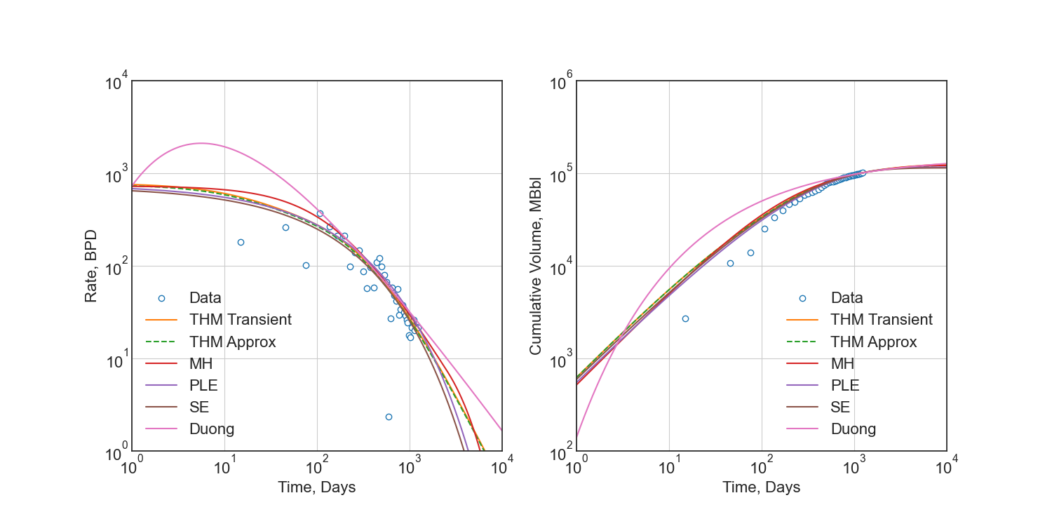
See the API documentation for a complete listing, detailed use examples, and model comparison.
Regression
No methods for regression are included in this library, as the models are simple enough to be implemented in any regression package. I recommend using scipy.optimize.least_squares.
For detailed derivation and argument for regression techniques, please see SPE-201404-MS Optimization Methods for Time–Rate–Pressure Production Data Analysis using Automatic Outlier Filtering and Bayesian Derivative Calculations. Additionally, you may view my blog post <https://dsfulf.github.io/blog/nonlin_reg/nonlin_reg.html>_ on the topic. The Jupyter Notebook is available here <https://github.com/dsfulf/blog/blob/master/nonlin_reg/nonlin_reg.ipynb>_.
The following is an example of how to use the THM model with scipy.optimize.least_squares.
from petbox import dca
import numpy as np
import scipy as sc

from scipy.optimize import least_squares

from typing import NamedTuple
from numpy.typing import NDArray


class Bounds(NamedTuple):
    qi: tuple[float, float]
    Di: tuple[float, float]
    bf: tuple[float, float]
    telf: tuple[float, float]


def load_data() -> tuple[NDArray[np.float64], NDArray[np.float64]]:
    ... # load your data here
    return rate, time


def filter_buildup(rate: NDArray[np.float64], time: NDArray[np.float64]) -> tuple[NDArray[np.float64], NDArray[np.float64]]:
    """Filter out buildup data"""
    idx = np.argmax(rate)
    return rate[idx:], time[idx:]


def jitter_rates(rate: NDArray[np.float64]) -> NDArray[np.float64]:
    """Add small jitter to rates to improve gradient descent"""
    # double-precion has at least 15 digits, so for rates in the 10_000s, this leaves a lot of room
    sd = 1e-6
    return rate * np.random.normal(1.0, sd, rate.shape)


def forecast_thm(params: NDArray[np.float64], time: NDArray[np.float64]) -> NDArray[np.float64]:
    """Forecast rates using the Transient Hyperbolic Model"""
    thm = dca.THM(
        qi=params[0],
        Di=params[1],
        bi=2.0,
        bf=params[2],
        telf=params[3],
        bterm=0.0,
        tterm=0.0
    )
    return thm.rate(time)


def log1sp(x: NDArray[np.float64]) -> NDArray[np.float64]:
    """Add small epsilon to avoid log(0) error"""
    return np.log(x + 1e-6)


def residuals(params: NDArray[np.float64], time: NDArray[np.float64], rate: NDArray[np.float64]) -> NDArray[np.float64]:
    """Residuals for scipy.optimize.least_squares"""
    forecast = forecast_thm(params, time)
    return log1sp(rate) - log1sp(forecast)


rate, time = load_data()
data_q = rate
data_t = time
rate, time = filter_buildup(rate, time)  # filter out buildup data
rate = jitter_rates(rate)  # add small jitter to rates to improve gradient descent
bounds = Bounds(  # these ***are not general***, they must be calibrated to your data
    qi=   (10.0,  10000.0),
    Di=   (1e-6,      0.8),
    bf=   ( 0.5,      1.5),
    telf= ( 5.0,     50.0)
)
opt = least_squares(
    fun=lambda params, time, rate: residuals(params, time, rate),  # residuals function
    bounds=list(zip(*bounds)),  # unpack bounds into list of tuples
    x0=[np.mean(p) for p in bounds],  # initial guess, mean works well enough
    args=(time, rate),  # additoinal arguments to `fun`
    loss='soft_l1',  # robust loss function
    f_scale=.35  # affects outlier senstivity of the regression, larger values are more sensitive
)

# no terminal segment
# bterm = 0.0
# tterm = 0.0

# hyperbolic terminal segment
bterm = 0.3
tterm = 15.0  # years

# exponential terminal segment
# bterm = 0.06  # 6.0% secant effective decline / year
# tterm = 0.0

params = np.r_[np.insert(opt.x, 2, 2.0), bterm, tterm]  # insert bi=2.0 and terminal parameters
print(params)
Which would print something like the following:
[1177.57885, 0.793357559, 2.0, 0.666515071, 7.17744813, 0.0, 0.0]
And passed into the THM constructor as follows:
thm = dca.THM.from_params(params)Development
petbox-dca is maintained by David S. Fulford (@dsfulf). Please post an issue or pull request in this repo for any problems or suggestions!
Version History
1.1.0
- Bug Fix
Fix bug in sign in MultisegmentHyperbolic.secant_from_nominal
- Other changes
Add mpmath to handle precision requires of THM transient functions (only required to use the functions)
Adjust default degree of THM transient function quadrature integration from 50 to 10 (scipy default is 5)
Update package versions for docs and builds
Address various floating point errors, suppress numpy warnings for those which are mostly unavoidable
Add test/doc_exapmles.py and update figures (not sure what happened to the old file)
Adjust range of values in tests to avoid numerical errors in numpy and scipy functions… these were near-epsilon impractical values anyway
1.0.8
- New functions
Added WaterPhase.wgr method
- Other changes
Adjust yield model rate function to return consistent units if primary phase is oil or gas
Update to numpy v1.20 typing
1.0.7
- Allow disabling of parameter checks by passing an interable of booleans, each indicating a check
to each model parameter.
Explicitly handle floating point overflow errors rather than relying on numpy.
1.0.6
- New functions
Added WaterPhase class
Added WaterPhase.wor method
Added PrimaryPhase.add_water method
- Other changes
A yield model may inherit both SecondaryPhase and WaterPhase, with the respective methods removed upon attachment to a PrimaryPhase.
1.0.5
- New functions
Bourdet algorithm
- Other changes
Update docstrings
Add bourdet data derivatives to detailed use examples
1.0.4
Fix typos in docs
1.0.3
Add documentation
Genericize numerical integration
Various refactoring
0.0.1 - 1.0.2
Internal releases
Release history Release notifications | RSS feed


Download files
Download the file for your platform. If you're not sure which to choose, learn more about installing packages.
Source Distribution
Built Distribution
Filter files by name, interpreter, ABI, and platform.
If you're not sure about the file name format, learn more about wheel file names.
Copy a direct link to the current filters
File details
Details for the file petbox_dca-1.1.2.tar.gz.
File metadata
- Download URL: petbox_dca-1.1.2.tar.gz
- Upload date:
- Size: 849.4 kB
- Tags: Source
- Uploaded using Trusted Publishing? No
- Uploaded via: twine/6.1.0 CPython/3.10.13
File hashes
| Algorithm | Hash digest | |
|---|---|---|
| SHA256 |
ac07aa42ca28318eda564e91a7f0a4ba0b5c582577261ba31176b0d4b1c19123
|
|
| MD5 |
e39299126c9883e99de8c555e19457a4
|
|
| BLAKE2b-256 |
67b6ef24fb3aafcf72dab32bbcb0bd71e016be7260164c523238df2b33a6c2e7
|
File details
Details for the file petbox_dca-1.1.2-py3-none-any.whl.
File metadata
- Download URL: petbox_dca-1.1.2-py3-none-any.whl
- Upload date:
- Size: 22.9 kB
- Tags: Python 3
- Uploaded using Trusted Publishing? No
- Uploaded via: twine/6.1.0 CPython/3.10.13
File hashes
| Algorithm | Hash digest | |
|---|---|---|
| SHA256 |
feb25011d0727fceb6b8dceae6c85a4023bf42b364d2fe51b51df3ee25261bc2
|
|
| MD5 |
9cf2d330de201713b10b051972261111
|
|
| BLAKE2b-256 |
b891ca6be6bfa49b2c51a78af5a600989aa70de474e2521a9e4921069f0873f4
|


