
photonviz
GPU-accelerated (WebGL2) charts for Jupyter, JupyterLab and Google Colab.






The Python bridge to Photon. NumPy arrays and torch tensors cross to the browser as binary buffers, so a million points still pan and zoom at 60fps inside a notebook cell — no image round-trip, no JSON blow-up.
pip install photonviz
Nothing else to install: the widget ships one self-contained ESM bundle, so there
is no CDN fetch, no jupyter labextension install, and no separate JS package.
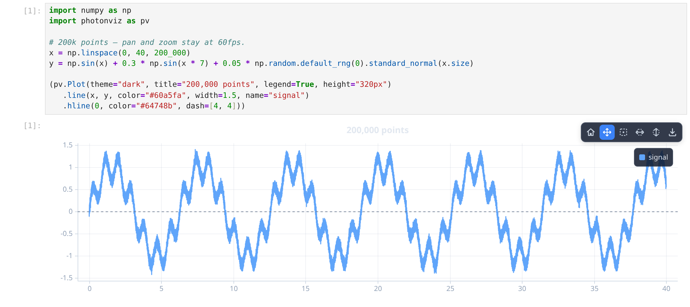
Real capture from JupyterLab — 200k points, interactive: wheel to zoom, drag to pan, hover for a tooltip.
Quick start
import numpy as np
import photonviz as pv

x = np.linspace(0, 10, 200_000)
pv.line(x, np.sin(x) + 0.3 * np.sin(x * 7), name="signal", plot={"theme": "dark", "legend": True})
Charts chain, and the last expression in a cell renders itself:
(pv.Plot(theme="dark", title="Two series", legend=True)
   .line(x, np.sin(x), name="sin", color="#60a5fa")
   .line(x, np.cos(x), name="cos", color="#f472b6", dash=[6, 4])
   .hline(0, color="#64748b"))
Every keyword maps 1:1 onto the TypeScript options,
so the JS reference applies verbatim — color, width, step, colorBy,
yAxis, renderType, and so on.
Google Colab
Run once per session, then use photonviz normally:
from google.colab import output
output.enable_custom_widget_manager()
What you can draw
pv.scatter(x, y, sizes=area, colors=hex_list)     # bubble chart
pv.histogram(samples, bins=40)
pv.heatmap(z, cols, rows, extent={"x": [0, 1], "y": [0, 1]}, colormap="magma")
pv.candlestick(t, o, h, l, c)                     # + heikin_ashi, bollinger, drawdown…
pv.regression(x, y, band=2)                       # OLS + confidence band (or method="loess")
pv.corr_matrix([a, b, c], names=["a", "b", "c"])  # diverging, locked to ±1
pv.psd(signal, sampleRate=1000)                   # Welch spectrum
pv.confusion_matrix(y_true, y_pred)               # + roc_curve, pr_curve, calibration, embedding…
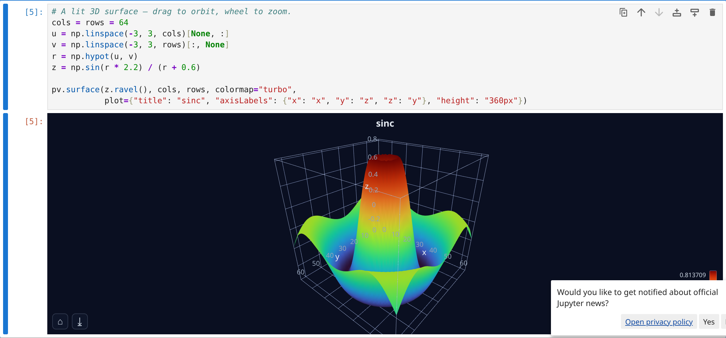
pv.surface(z, cols, rows)                         # 3D — orbit with the mouse
pv.polar_line(theta, r)
Plot, Plot3D and Polar are the full objects; the module-level names are
one-line shortcuts. Pass plot={...} to a shortcut to configure the plot itself:
pv.scatter(x, y, size=4, plot={"theme": "dark", "pick": "xy", "colorbar": False})
Model architecture
Hand a PyTorch, Keras, scikit-learn or ONNX model straight to
model_graph — the export happens in Python, the layout in the browser.
import torch, torchvision, photonviz as pv

model = torchvision.models.resnet18()

# 2D — a Netron-style DAG, with residual connections routed around the trunk.
pv.model_graph(model, example_input=torch.randn(1, 3, 224, 224), direction="horizontal")

# 3D — one cuboid per layer, sized from its output tensor: feature maps shrink
# while channel depth grows.
pv.model_graph_3d(
    model,
    example_input=torch.randn(1, 3, 224, 224),
    labels="full",
    plot={"aspectMode": "data", "projection": "orthographic", "showAxes": False},
)
| Framework | How it is read | Notes |
|---|---|---|
| PyTorch | torch.fx symbolic trace |
Branches and skip connections survive. Pass example_input= to record shapes. Untraceable models fall back to a flat chain of leaf modules. |
| Keras / TF | model.to_json() + per-layer shapes |
Sequential and functional, Keras 2 and 3. |
| scikit-learn | Pipeline / ColumnTransformer / FeatureUnion walk |
Parallel branches fan out and back in. An MLPClassifier expands into its real dense stack. |
| ONNX | MessageToDict + shape inference |
The framework-neutral path. |
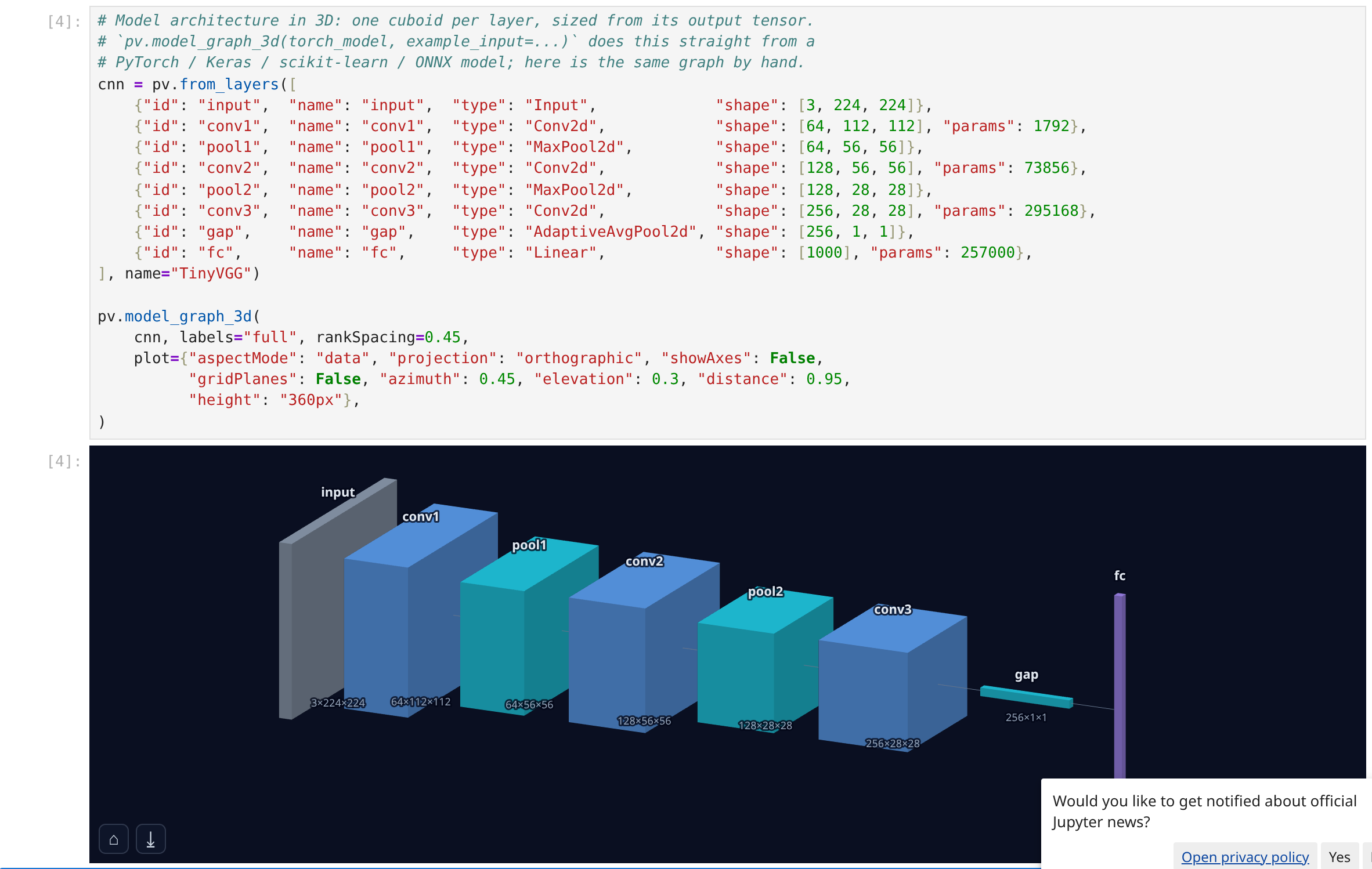
Each cuboid is one layer: the visible face is its feature map, the thickness its channel count. Drag to orbit.
The exporters are usable on their own — pv.from_torch(model), pv.from_keras,
pv.from_sklearn, pv.from_onnx — and a hand-written
{"nodes": [...], "edges": [...]} graph works too.
Example notebooks
Runnable, in the repo — examples/notebooks/:
| Notebook | What it covers |
|---|---|
quickstart.ipynb |
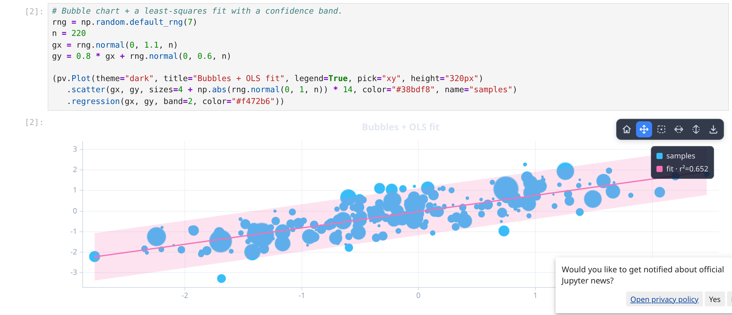
The five-minute tour: a 200k-point line, a bubble chart with an OLS fit, a confusion matrix, a 3D model graph, a 3D surface. |
gallery.ipynb |
The full spread — distributions, fields, custom colours, finance, signal processing, ML metrics, model architecture, and 3D. |
How it works
photonviz is an anywidget, which is why the same
object renders in Jupyter Notebook 7, JupyterLab 4, VS Code and Colab with no
per-frontend code.
Chart calls build a plain dict. On sync, every array-like is swapped for a
{"$buffer": i} marker and its raw bytes are appended to a buffer list;
ipywidgets ships those as binary. The browser rebuilds typed-array views over
them and hands them to @photonviz/core, which uploads straight to GPU buffers.
Colours, names, extents and other structural values stay JSON.
All plots on a page share one WebGL2 context, so a notebook with dozens of charts will not exhaust the browser's context limit.
Development
From a checkout of the monorepo:
pnpm install
pnpm build:python          # bundles the widget into src/photonviz/static/widget.js
cd python
pip install -e ".[dev]"
pytest
License
MIT
1 maintainer

Download files
Download the file for your platform. If you're not sure which to choose, learn more about installing packages.
Source Distribution
Built Distribution
Filter files by name, interpreter, ABI, and platform.
If you're not sure about the file name format, learn more about wheel file names.
Copy a direct link to the current filters
File details
Details for the file photonviz-0.7.0.tar.gz.
File metadata
- Download URL: photonviz-0.7.0.tar.gz
- Upload date:
- Size: 112.7 kB
- Tags: Source
- Uploaded using Trusted Publishing? No
- Uploaded via:
twine/6.2.0 CPython/3.11.15
File hashes
| Algorithm | Hash digest | |
|---|---|---|
| SHA256 |
77fd8e6ec884d9bb0d211dc73c329f529562b0087022caeeeab3be5ff0d2ca4a
|
|
| MD5 |
41c6471d0d770066794df0bc75601124
|
|
| BLAKE2b-256 |
9e551781538840936bc80eee0c18cacfb287458ddac18290c609ec6735239eaa
|
File details
Details for the file photonviz-0.7.0-py3-none-any.whl.
File metadata
- Download URL: photonviz-0.7.0-py3-none-any.whl
- Upload date:
- Size: 116.1 kB
- Tags: Python 3
- Uploaded using Trusted Publishing? No
- Uploaded via:
twine/6.2.0 CPython/3.11.15
File hashes
| Algorithm | Hash digest | |
|---|---|---|
| SHA256 |
19e3c04cac82e4330915c48e1ba80f57ca66444e88744c5a3eb9dc5739d4c5a7
|
|
| MD5 |
dd7c6fd7f9007134b7ab8ec1ded77ce1
|
|
| BLAKE2b-256 |
e4e836ae93a29e0527ed20f9a1fdfc99c7fc59cf1e4eba942212bcfebcc4efff
|














