
$\Phi$-SO : Physical Symbolic Optimization








Source code: WassimTenachi/PhySO
Documentation: physo.readthedocs.io
What's New ✨
2025-08 : 📦 Install via pip install physo and conda now available!
2025-07 : 🐍 Python 3.12 + latest NumPy/PyTorch/SymPy support.
2024-06 : 📚 Full documentation overhaul.
2024-05 : 🔬 Class SR: Multi-dataset symbolic regression.
2024-02 : 🎯 Uncertainty-aware fitting.
2023-08 : ⚡ Dimensional analysis acceleration.
2023-03 : 🌟 PhySO initial release (physics-focused SR).
Highlights
$\Phi$-SO's symbolic regression module uses deep reinforcement learning to infer analytical physical laws that fit data points, searching in the space of functional forms.
physo is able to leverage:
-
Physical units constraints, reducing the search space with dimensional analysis ([Tenachi et al 2023])
-
Class constraints, searching for a single analytical functional form that accurately fits multiple datasets - each governed by its own (possibly) unique set of fitting parameters ([Tenachi et al 2024])
$\Phi$-SO recovering the equation for a damped harmonic oscillator:
https://github.com/WassimTenachi/PhySO/assets/63928316/655b0eea-70ba-4975-8a80-00553a6e2786
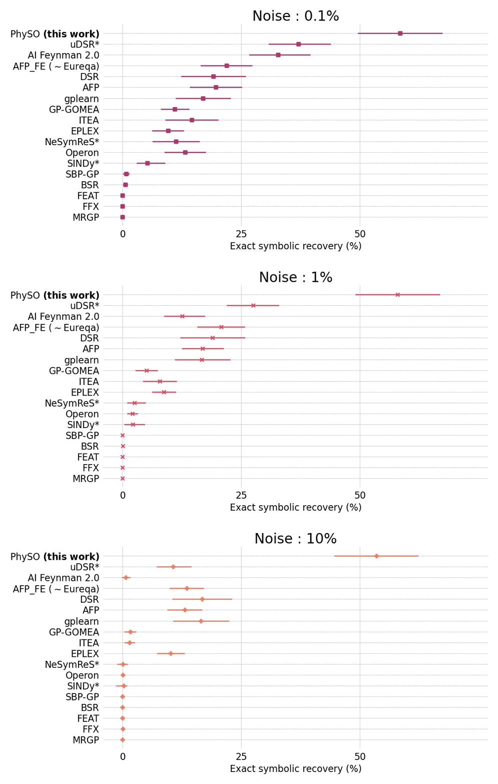
Performances on the standard Feynman benchmark from SRBench) comprising 120 expressions from the Feynman Lectures on Physics against popular SR packages.
$\Phi$-SO achieves state-of-the-art performance in the presence of noise (exceeding 0.1%) and shows robust performances even in the presence of substantial (10%) noise:
Installation
The package has been tested on:
- Linux
- OSX (ARM & Intel)
- Windows
If you are encountering issues with the installation, installing from the source should help. If you are still having issues, please refer to the FAQ or raise an issue on the GitHub repository.
Installing with pip
Installing physo from PyPI :
pip install physo
Installing with conda
Installing physo using conda:
conda install -c conda-forge physo
Getting started (SR)
In this tutorial, we show how to use physo to perform Symbolic Regression (SR).
The reference notebook for this tutorial can be found here: sr_quick_start.ipynb.
Setup
Importing the necessary libraries:
# External packages
import numpy as np
import matplotlib.pyplot as plt
import torch
Importing physo:
# Internal code import
import physo
import physo.learn.monitoring as monitoring
It is recommended to fix the seed for reproducibility:
# Seed
seed = 0
np.random.seed(seed)
torch.manual_seed(seed)
Making synthetic datasets
Making a toy synthetic dataset:
# Making toy synthetic data
z = np.random.uniform(-10, 10, 50)
v = np.random.uniform(-10, 10, 50)
X = np.stack((z, v), axis=0)
y = 1.234*9.807*z + 1.234*v**2
It should be noted that free constants search starts around 1. by default. Therefore when using default hyperparameters, normalizing the data around an order of magnitude of 1 is strongly recommended.
DA side notes:
$\Phi$-SO can exploit DA (dimensional analysis) to make SR more efficient.
On can consider the physical units of $X=(z,v)$, $z$ being a length of dimension $L^{1}, T^{0}, M^{0}$, v a velocity of dimension $L^{1}, T^{-1}, M^{0}$, $y=E$ if an energy of dimension $L^{2}, T^{-2}, M^{1}$.
If you are not working on a physics problem and all your variables/constants are dimensionless, do not specify any of the xx_units arguments (or specify them as [0,0] for all variables/constants) and physo will perform a dimensionless symbolic regression task.
Datasets plot:
n_dim = X.shape[0]
fig, ax = plt.subplots(n_dim, 1, figsize=(10,5))
for i in range (n_dim):
    curr_ax = ax if n_dim==1 else ax[i]
    curr_ax.plot(X[i], y, 'k.',)
    curr_ax.set_xlabel("X[%i]"%(i))
    curr_ax.set_ylabel("y")
plt.show()
SR configuration
It should be noted that SR capabilities of physo are heavily dependent on hyperparameters, it is therefore recommended to tune hyperparameters to your own specific problem for doing science.
Summary of currently available hyperparameters presets configurations:
| Config | Recommended usecases | Speed | Effectiveness | Notes |
|---|---|---|---|---|
config0 |
Demos | ★★★ | ★ | Light and fast config. |
config1 |
SR with DA $^$ ; Class SR with DA $^$ | ★ | ★★★ | Config used for Feynman Benchmark and MW streams Benchmark. |
config2 |
SR ; Class SR | ★★ | ★★ | Config used for Class Benchmark. |
$^*$ DA = Dimensional Analysis
Users are encouraged to edit configurations (they can be found in: physo/config/).
By default, config0 is used, however it is recommended to follow the upper recommendations for doing science.
DA side notes:
- During the first tens of iterations, the neural network is typically still learning the rules of dimensional analysis, resulting in most candidates being discarded and not learned on, effectively resulting in a much smaller batch size (typically 10x smaller), thus making the evaluation process much less computationally expensive. It is therefore recommended to compensate this behavior by using a higher batch size configuration which helps provide the neural network sufficient learning information.
Logging and visualisation setup:
save_path_training_curves = 'demo_curves.png'
save_path_log             = 'demo.log'

run_logger     = lambda : monitoring.RunLogger(save_path = save_path_log,
                                                do_save = True)

run_visualiser = lambda : monitoring.RunVisualiser (epoch_refresh_rate = 1,
                                           save_path = save_path_training_curves,
                                           do_show   = False,
                                           do_prints = True,
                                           do_save   = True, )
Running SR
Given variables data $(x_0,..., x_n)$ (here $(z, v)$ ), the root variable $y$ (here $E$) as well as free and fixed constants, you can run an SR task to recover $f$ via the following command.
DA side notes:
Here we are allowing the use of a fixed constant $1$ of dimension $L^{0}, T^{0}, M^{0}$ (ie dimensionless) and free constants $m$ of dimension $L^{0}, T^{0}, M^{1}$ and $g$ of dimension $L^{1}, T^{-2}, M^{0}$.
It should be noted that here the units vector are of size 3 (eg: [1, 0, 0]) as in this example the variables have units dependent on length, time and mass only.
However, units vectors can be of any size $\leq 7$ as long as it is consistent across X, y and constants, allowing the user to express any units (dependent on length, time, mass, temperature, electric current, amount of light, or amount of matter).
In addition, dimensional analysis can be performed regardless of the order in which units are given, allowing the user to use any convention ([length, mass, time] or [mass, time, length] etc.) as long as it is consistent across X,y and constants.
# Running SR task
expression, logs = physo.SR(X, y,
                            # Giving names of variables (for display purposes)
                            X_names = [ "z"       , "v"        ],
                            # Associated physical units (ignore or pass zeroes if irrelevant)
                            X_units = [ [1, 0, 0] , [1, -1, 0] ],
                            # Giving name of root variable (for display purposes)
                            y_name  = "E",
                            y_units = [2, -2, 1],
                            # Fixed constants
                            fixed_consts       = [ 1.      ],
                            fixed_consts_units = [ [0,0,0] ],
                            # Free constants names (for display purposes)
                            free_consts_names = [ "m"       , "g"        ],
                            free_consts_units = [ [0, 0, 1] , [1, -2, 0] ],
                            # Symbolic operations that can be used to make f
                            op_names = ["mul", "add", "sub", "div", "inv", "n2", "sqrt", "neg", "exp", "log", "sin", "cos"],
                            get_run_logger     = run_logger,
                            get_run_visualiser = run_visualiser,
                            # Run config
                            run_config = physo.config.config0.config0,
                            # Parallel mode (only available when running from python scripts, not notebooks)
                            parallel_mode = False,
                            # Number of iterations
                            epochs = 20
)
Inspecting the best expression found
Getting best expression:
The best expression found (in accuracy) is returned in the expression variable:
best_expr = expression
print(best_expr.get_infix_pretty())
>>>
                     2
    -g⋅m⋅z + -v⋅v⋅sin (1.0)⋅1.0⋅m
It can also be loaded later on from log files:
import physo
from physo.benchmark.utils import symbolic_utils as su
import sympy

# Loading pareto front expressions
pareto_expressions = physo.read_pareto_pkl("demo_curves_pareto.pkl")
# Most accurate expression is the last in the Pareto front:
best_expr = pareto_expressions[-1]
print(best_expr.get_infix_pretty())
Display:
The expression can be converted into...
A sympy expression:
best_expr.get_infix_sympy()
>>> -g*m*z - v*v*sin(1.0)**2*1.0*m
A sympy expression (with evaluated free constants values):
best_expr.get_infix_sympy(evaluate_consts=True)[0]
>>> 1.74275713004454*v**2*sin(1.0)**2 + 12.1018380702846*z
A latex string:
best_expr.get_infix_latex()
>>> '\\frac{m \\left(- 1000000000000000 g z - 708073418273571 v^{2}\\right)}{1000000000000000}'
A latex string (with evaluated free constants values):
sympy.latex(best_expr.get_infix_sympy(evaluate_consts=True))
>>> '\\mathtt{\\text{[1.74275713004454*v**2*sin(1.0)**2 + 12.1018380702846*z]}}'
Getting free constant values:
best_expr.free_consts
>>> FreeConstantsTable
     -> Class consts (['g' 'm']) : (1, 2)
     -> Spe consts   ([]) : (1, 0, 1)
best_expr.free_consts.class_values
>>> tensor([[ 6.9441, -1.7428]], dtype=torch.float64)
Checking exact symbolic recovery
# To sympy
best_expr = best_expr.get_infix_sympy(evaluate_consts=True)

best_expr = best_expr[0]

# Printing best expression simplified and with rounded constants
print("best_expr : ", su.clean_sympy_expr(best_expr, round_decimal = 4))

# Target expression was:
target_expr = sympy.parse_expr("1.234*9.807*z + 1.234*v**2")
print("target_expr : ", su.clean_sympy_expr(target_expr, round_decimal = 4))

# Check equivalence
print("\nChecking equivalence:")
is_equivalent, log = su.compare_expression(
                        trial_expr  = best_expr,
                        target_expr = target_expr,
                        handle_trigo            = True,
                        prevent_zero_frac       = True,
                        prevent_inf_equivalence = True,
                        verbose                 = True,
)
print("Is equivalent:", is_equivalent)
>>> best_expr :  1.234*v**2 + 12.1018*z
    target_expr :  1.234*v**2 + 12.1018*z

    Checking equivalence:
      -> Assessing if 1.234*v**2 + 12.101838*z (target) is equivalent to 1.74275713004454*v**2*sin(1.0)**2 + 12.1018380702846*z (trial)
       -> Simplified expression : 1.23*v**2 + 12.1*z
       -> Symbolic error        : 0
       -> Symbolic fraction     : 1
       -> Trigo symbolic error        : 0
       -> Trigo symbolic fraction     : 1
       -> Equivalent : True
    Is equivalent: True
Documentation
Further documentation can be found at physo.readthedocs.io.
Quick start guide for Symbolic Regression : HERE
Quick start guide for Class Symbolic Regression : HERE
Citing this work
Symbolic Regression with reinforcement learning & dimensional analysis
@ARTICLE{PhySO_RL_DA,
       author = {{Tenachi}, Wassim and {Ibata}, Rodrigo and {Diakogiannis}, Foivos I.},
        title = "{Deep Symbolic Regression for Physics Guided by Units Constraints: Toward the Automated Discovery of Physical Laws}",
      journal = {ApJ},
         year = 2023,
        month = dec,
       volume = {959},
       number = {2},
          eid = {99},
        pages = {99},
          doi = {10.3847/1538-4357/ad014c},
archivePrefix = {arXiv},
       eprint = {2303.03192},
 primaryClass = {astro-ph.IM},
       adsurl = {https://ui.adsabs.harvard.edu/abs/2023ApJ...959...99T},
      adsnote = {Provided by the SAO/NASA Astrophysics Data System}
}
Class Symbolic Regression
@ARTICLE{PhySO_ClassSR,
       author = {{Tenachi}, Wassim and {Ibata}, Rodrigo and {Fran{\c{c}}ois}, Thibaut L. and {Diakogiannis}, Foivos I.},
        title = "{Class Symbolic Regression: Gotta Fit 'Em All}",
      journal = {The Astrophysical Journal Letters},
         year = {2024},
        month = {jul},
       volume = {969},
       number = {2},
          eid = {arXiv:2312.01816},
        pages = {L26},
          doi = {10.3847/2041-8213/ad5970},
archivePrefix = {arXiv},
       eprint = {2312.01816},
 primaryClass = {cs.LG},
       adsurl = {https://ui.adsabs.harvard.edu/abs/2023arXiv231201816T},
      adsnote = {Provided by the SAO/NASA Astrophysics Data System}
}
2 maintainers


Metadata
2 maintainers
Release files for physo 1.1.11
For a detailed explanation of source distributions (sdists) and built distributions (wheels), please see the package formats documentation.
Source distribution (sdist)
| File | Size | Uploaded | |
|---|---|---|---|
| physo-1.1.11.tar.gz | 205.0 kB | Details |
Built distribution (wheel)
| File | Interpreter | ABI | Platform | Reset |
|---|---|---|---|---|
| physo-1.1.11-py3-none-any.whl | Python 3 | none | any | Details |
Total release size: 440.8 kB
Release files / physo-1.1.11.tar.gz
| Download URL | physo-1.1.11.tar.gz |
|---|---|
| Size | 205.0 kB |
| Tags | Source |
|
SHA-256 checksum How to use checksums |
97b656dc74904650790236253fb8ba6c7f56ef02a180acd2801fbb166019fdb4
|
|
BLAKE2b-256 checksum How to use checksums |
bc59a48b72caadc82b6f6ab7fb5d69b244f3cb08f52048e44e7de4f75e348f4e
|
| Upload date | |
|
Uploaded using Trusted Publishing? What is trusted publishing? |
No |
| Uploaded via |
twine/6.1.0 CPython/3.12.11
|
Release files / physo-1.1.11-py3-none-any.whl
| Download URL | physo-1.1.11-py3-none-any.whl |
|---|---|
| Size | 235.8 kB |
| Tags | Python 3 |
|
SHA-256 checksum How to use checksums |
1deb9e85ac163a9619f3b4ba68743827ddc14b1a51e236092bb99ee1a7c77bff
|
|
BLAKE2b-256 checksum How to use checksums |
c31e56106bcb1078cc4863a8ebfc26d5f0c054d76bb98022e0a6e5aa0c8dc56b
|
| Upload date | |
|
Uploaded using Trusted Publishing? What is trusted publishing? |
No |
| Uploaded via |
twine/6.1.0 CPython/3.12.11
|














