



Installation · Quick Start · Examples · Extending pinnse · Citation
Table of Contents
- What is pinnse?
- Why Use Physics-Informed Surrogate Models?
- Installation
- Quick Start
- Framework Overview
- Walkthrough: Training a PINN Surrogate
- Core Package API
- Normalization Strategies
- Example Case Studies
- Repository Structure
- Extending pinnse to a New Process
- Citation
- Contributing
- License
What is pinnse?
pinnse is a Python package that makes it straightforward to develop physics-informed neural-network (PINN) surrogate models for chemical process systems. It separates the reusable machine-learning infrastructure — data handling, normalization, neural-network construction, training, checkpointing, and visualization — from the process-specific ingredients that you define once for each system: operating bounds, governing equations, and residual formulations.
The core idea is simple:
- Define the process physics as residual functions (material balances, energy balances, equilibrium relations).
- Train a differentiable neural-network surrogate against both labelled data and those physical constraints.
- Obtain a fast, physically consistent model suitable for simulation, design, or optimization.
The repository includes ready-to-run examples covering:
- Nonideal flash separation (vapor–liquid equilibrium)
- Isothermal plug-flow reactors under multiple surrogate formulations (effluent flowrates, reaction extents, conversions)
- Inverse PINNs for kinetic parameter estimation
- Nonisothermal plug-flow reactors with coupled mass and energy balances
- Noisy measurement data, comparing PINNs with purely data-driven networks trained on the same noisy labels
- Dynamic processes, with a recurrent PINN that predicts the state trajectory of a nonisothermal CSTR
Why Use Physics-Informed Surrogate Models?
First-principles models in chemical engineering — reactor balances, phase equilibrium, heat transfer — are often nonlinear, tightly coupled, and expensive to solve repeatedly in optimization, control, or uncertainty-quantification loops.
Purely data-driven surrogates can approximate these models cheaply, but they come with a critical drawback: they can violate conservation laws, equilibrium relationships, or boundary conditions, especially when extrapolating beyond the training data.
Physics-informed neural networks address this by adding soft physical constraints directly into the training loss. During training, the network is penalized not only for mismatch with labelled data, but also for violating the governing equations at a set of collocation points sampled across the input domain. The result is a surrogate that is:
- Data-efficient — physical constraints reduce the amount of labelled data needed.
- Physically consistent — conservation laws and boundary conditions are respected.
- Differentiable — the surrogate and its gradients are available analytically through automatic differentiation, which is useful for sensitivity analysis and gradient-based optimization.
Installation
Basic install
pip install pinnse
This installs the core dependencies: PyTorch, NumPy, SciPy, pandas, tqdm, scikit-learn, matplotlib, and openpyxl.
Verify the installation:
python -c "from pinnse import ANN, DataModule, Training; print('pinnse is ready')"
Recommended: use a clean environment
conda create -n pinnse python=3.11 -y
conda activate pinnse
pip install pinnse
Development install (to run examples or modify the source)
git clone https://github.com/hverma99/pinnse.git
cd pinnse
pip install -e ".[dev]"
GPU support
Training PINNs is compute-intensive and a CUDA-enabled GPU is strongly recommended. pip install pinnse installs the default (CPU) PyTorch build. To enable GPU acceleration, install the appropriate PyTorch build for your CUDA version before or after installing pinnse:
# Example: PyTorch with CUDA 12.6 (check https://pytorch.org/get-started for your version)
pip install torch --index-url https://download.pytorch.org/whl/cu126
pinnse automatically uses the GPU when available. All example scripts include:
device = torch.device("cuda" if torch.cuda.is_available() else "cpu")
Optional: Aspen Plus integration
Flash-separation data generation uses Aspen Plus COM automation (Windows only). To install the optional dependency:
pip install "pinnse[aspen]"
Note: Aspen Plus is only needed to regenerate flash datasets. All supplied
.xlsxdatasets can be used for training without Aspen.
Quick Start
Use pinnse in Python
import torch.nn as nn
from pinnse import ANN

# Build a feedforward PINN: 5 inputs → 3 hidden layers (64 neurons each) → 3 outputs
model = ANN(layer_size=[5, 64, 64, 64, 3], activation=nn.Tanh)
Run a complete example from the repository
The isothermal PFR example is the fastest way to see pinnse in action — it is self-contained and does not require Aspen Plus.
git clone https://github.com/hverma99/pinnse.git
cd pinnse/examples/isopfr/efm

python main.py     # Train the PINN surrogate
python check.py    # Evaluate and compare against first-principles solution
This will:
- Load labelled input/output data (
I_S_data.xlsx,D_S_data.xlsx) - Normalize the input and output spaces
- Construct supervised, physics-collocation, and boundary-collocation data loaders
- Build and train a PINN surrogate with data + physics + boundary losses
- Checkpoint the best model to
logs/ - Evaluate the trained model and generate comparison figures
Framework Overview
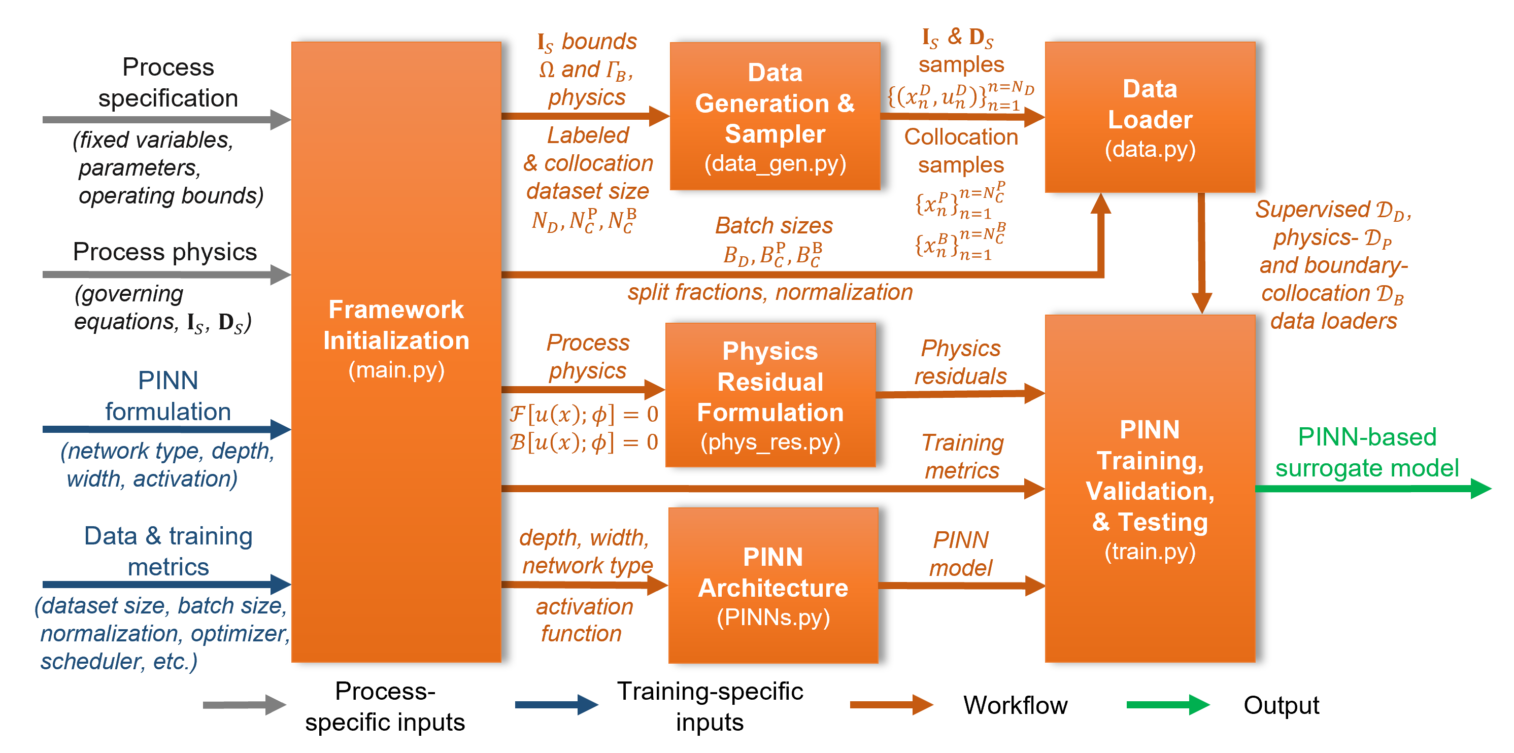
pinnse trains a neural-network surrogate by minimizing a composite loss that combines supervised data fitting with physics-based regularization. The total loss has three components:
- Data loss — fits the network predictions to labelled input/output samples from a process simulator or experiment.
- Physics loss — penalizes violations of governing equations (e.g., material balances, energy balances) evaluated at collocation points sampled across the input domain.
- Boundary loss — enforces boundary or initial conditions (e.g., inlet conditions for a PFR at reactor volume = 0).
The physics and boundary losses are weighted by tunable coefficients that can be fixed or updated adaptively during training, either by the built-in gradient-norm balancing or by a rule you supply. Alternatively, a gradient aggregator such as PCGrad can combine the individual loss gradients directly (see Custom loss weighting and gradient aggregation).
Each example in the repository follows a consistent workflow, organized across a small set of files:
| Stage | What happens | File |
|---|---|---|
| Setup | Define process variables, operating bounds, architecture, optimizer, loss weights | main.py |
| Data generation | Generate labelled data from Aspen Plus, SciPy ODE solvers, or other process models | data_gen.py |
| Data loading | Split labelled data; construct supervised, physics-collocation, and boundary-collocation loaders | pinnse/data.py |
| Architecture | Build the differentiable neural-network surrogate | pinnse/PINNs.py |
| Physics residuals | Encode governing equations in residual form | phys_res.py |
| Training | Optimize with Adam (+ optional L-BFGS refinement); checkpoint best model | pinnse/train.py |
| Evaluation | Load trained model, denormalize outputs, compute error metrics, generate figures | check.py |
Walkthrough: Training a PINN Surrogate
This walkthrough uses the isothermal PFR — effluent flowrate model (EFM) example. The full code is in examples/isopfr/efm/main.py.
Step 1: Load and normalize data
import pandas as pd
from pinnse import Normalization

I_S_data = pd.read_excel("I_S_data.xlsx")   # Inputs:  inlet flowrates, P, T, V
D_S_data = pd.read_excel("D_S_data.xlsx")   # Outputs: outlet flowrates

# Normalize to [-1, 1] with formulation-aware scaling
norm_I_S, norm_D_S, I_S_metrics, D_S_metrics = Normalization.min_max_pfr(
    I_S_data=I_S_data,
    D_S_data=D_S_data,
    formulation="EFM",
    species=["O2", "CO2", "H2O", "C6H6", "C4H2O3"],
)
Step 2: Create data loaders
from pinnse import DataModule

data = DataModule(
    I_S_data=norm_I_S,
    D_S_data=norm_D_S,
    labeled_data_batch_size=500,
    physics_coll_data_size=20000,     # Number of collocation points
    physics_coll_batch_size=500,
    boundary_coll_data_size=5000,
    boundry_coll_batch_size=1000,
    test_frac=0.1,
    val_frac=0.1,
)

train_loader, val_loader, test_loader = data.labeled_data_loader()
phys_coll_loader = data.phys_colloc_loader()    # LHS + Dirichlet sampling
bnd_coll_loader  = data.bnd_colloc_loader()     # Boundary-fixed sampling
Step 3: Define physics and boundary residuals
These are defined in a separate phys_res.py file (process-specific). The residual classes are callables with signature (x, y) → residual_tensor, where x is the normalized input batch and y is the network output.
from phys_res import Physics, Boundary

physics  = Physics(I_S_metrics, D_S_metrics, species, nu, key_species, k, E)
boundary = Boundary(species)
Step 4: Build the model
import torch, torch.nn as nn
from pinnse import ANN

dim_in = I_S_data.shape[1]   # Number of input features
dim_ot = D_S_data.shape[1]   # Number of output targets

layer_size = [dim_in] + [64] * 6 + [dim_ot]   # 6 hidden layers, 64 neurons
model = ANN(layer_size, activation=nn.Tanh).to(device)
Step 5: Train
from pinnse import Training

training = Training(
    model=model,
    train_loader=train_loader,
    val_loader=val_loader,
    test_loader=test_loader,
    optimizer=torch.optim.Adam(model.parameters(), lr=1e-4),
    loss_fn=nn.MSELoss(),
    device=device,
    phys_coll_loader=phys_coll_loader,
    bnd_coll_loader=bnd_coll_loader,
    phys_residual=physics,
    bnd_residual=boundary,
    ckpt_path="./logs/best_model.pth",
    phys_weight=1.0,      # Weight for physics loss
    bnd_weight=1.0,       # Weight for boundary loss
    adapt_wts=False,       # Set True for adaptive gradient-norm balancing
)

history = training.adam_step(epochs=75000, val_every=100)
For problems that benefit from second-order optimization, append an L-BFGS refinement stage:
history_lbfgs = training.lbfgs_step(mode="combined", N_LBFGS=150)
Step 6: Save and visualize
from pinnse import Save, Plotter

Save.excel(history)
Save.csv(history)

plots = Plotter(history=history, val_every=100)
plots.plot_everything(savepath="figures/", scale=1000)
Core Package API
All public classes are importable directly from pinnse:
from pinnse import (
    ANN, SANN, MultiHeadANN, Fourier_ANN,   # Feedforward architectures
    RecurrentANN,                            # Sequence architecture
    DataModule, SequenceDataModule,          # Data loading
    Training, PCGrad,                        # Training loop, gradient aggregation
    Plotter,                                 # Visualization
    Normalization, Denormalization,          # Scaling
    Save, Analyze, Noise,                    # Utilities
)
Neural-Network Architectures (pinnse/PINNs.py)
| Class | Description | When to use |
|---|---|---|
ANN |
Fully connected feedforward network. Xavier-uniform weight init, zero biases. | General-purpose PINN surrogate. Default choice. |
SANN |
Same as ANN but applies Softplus to the output layer. |
When outputs must be non-negative (concentrations, flowrates). |
MultiHeadANN |
Shared trunk with multiple independent output heads. | When outputs group naturally (e.g., compositions vs. temperature) and benefit from shared representation with separate specialization. |
Fourier_ANN |
Feedforward network with sinusoidal Fourier-feature embedding on the last input coordinate. | When the target function varies rapidly or has multi-scale behavior along one input dimension (e.g., reactor length). |
RecurrentANN |
Recurrent sequence-to-sequence network (cell="rnn", "gru" or "lstm"; stacked with n_layers) with an output head applied at each time step (head_layers). Maps inputs of shape (batch, seq_len, in_dim) to outputs of shape (batch, seq_len, out_dim). |
Dynamic processes, where the surrogate predicts a whole state trajectory from an initial condition and an input schedule. Use with SequenceDataModule. |
RecurrentANN starts from a zero hidden state, so the initial condition must be supplied as input features (typically held constant along the sequence). Its forward pass takes a single tensor, so it works in the same Training loop as the feedforward networks.
Data Handling (pinnse/data.py)
DataModule converts normalized DataFrames into PyTorch data loaders for the three loss components.
| Method | Purpose |
|---|---|
labeled_data_loader() |
Splits labelled data into train/validation/test DataLoader objects. |
phys_colloc_loader() |
Generates physics-collocation points using Latin Hypercube Sampling (LHS). Composition variables (prefixed Z_, X_, Y_) are sampled from Dirichlet distributions so mole fractions sum to 1. |
bnd_colloc_loader() |
Generates boundary-collocation points with one input fixed (e.g., reactor volume = 0 for inlet conditions). |
inspect_loader() |
Prints loader summary (batch shapes, number of batches). |
save_loaders() |
Exports loader contents to Excel for inspection. |
SequenceDataModule is the counterpart of DataModule for trajectory data, where each sample is a whole trajectory rather than an independent row.
| Feature | Behavior |
|---|---|
| Input format | Normalized NumPy arrays of shape (n_trajectories, seq_len, n_features) for both I_S_data and D_S_data. |
labeled_data_loader() |
Splits by whole trajectory, so no trajectory contributes to more than one of the train/validation/test partitions. labeled_data_batch_size counts trajectories. |
phys_colloc_loader() |
Generates collocation trajectories by Latin Hypercube Sampling. Context features (constant along a trajectory, such as the initial condition) are sampled once per trajectory. Driving features (such as a coolant temperature) are sampled as n_segments levels and expanded into a piecewise-constant schedule. |
context_cols |
Indices of the context features. If omitted, they are detected as the features that never vary within a trajectory. |
With sequence data, the physics residual receives the input and output sequences, x of shape (batch, seq_len, dim_in) and y of shape (batch, seq_len, dim_ot), so it can enforce a discrete-time relation between successive predicted states. There is no boundary-collocation loader: initial conditions enter through the context features.
import torch.nn as nn
from pinnse import RecurrentANN, SequenceDataModule

# norm_I_S: (n_trajectories, 200, 3), features [CA_0, T_0, TC_k], normalized
# norm_D_S: (n_trajectories, 200, 2), features [CA_k1, T_k1], normalized
data = SequenceDataModule(
    I_S_data=norm_I_S,
    D_S_data=norm_D_S,
    labeled_data_batch_size=64,     # trajectories per batch
    physics_coll_data_size=1000,    # collocation trajectories
    physics_coll_batch_size=64,
    n_segments=4,                   # piecewise-constant coolant schedule
    test_frac=0.1,
    val_frac=0.1,
)

train_loader, val_loader, test_loader = data.labeled_data_loader()
phys_coll_loader = data.phys_colloc_loader()

model = RecurrentANN(in_dim=3, hidden_dim=64, out_dim=2, cell="gru", head_layers=[64])
The full workflow, including the unrolled discrete-time residual, is in examples/dynamic.cstr.
Training (pinnse/train.py)
The Training class manages the full training loop.
| Method | Purpose |
|---|---|
adam_step(epochs, val_every) |
First-order training with Adam. Validates periodically and checkpoints the best model. |
lbfgs_step(mode, N_LBFGS) |
Second-order refinement with L-BFGS (full-batch, strong Wolfe line search). Modes: "data", "physics", "boundary", "combined", "overall physics". |
validate_test(loader) |
Evaluate data, physics, and boundary losses on a given loader. |
Key constructor parameters:
| Parameter | Description |
|---|---|
phys_weight, bnd_weight |
Scalar weights for physics and boundary losses. Set to 0.0 to disable. |
adapt_wts |
If True, automatically adjusts phys_weight and bnd_weight every 10 epochs based on gradient-norm balancing. Requires both weights to be nonzero. |
theta |
An nn.Parameter for inverse problems — trainable physical parameters (e.g., activation energies) that are optimized alongside network weights. |
weight_scheme |
Optional callable (grad_d, grad_p, grad_b) -> (w_phys, w_bnd) that replaces the built-in adaptive-weight rule. Used only when adapt_wts=True and both weights are nonzero. |
grad_aggregator |
Optional callable that combines the per-loss gradients itself, replacing the default weighted-sum update. PCGrad() is provided. |
Custom loss weighting and gradient aggregation
By default, with adapt_wts=True, every 10 epochs each weight is moved toward the ratio of the data-loss gradient norm to its own loss's gradient norm, smoothed by an exponential moving average (factor 0.1). To use a different rule, pass weight_scheme. It receives the average gradient norms of the data, physics and boundary losses over the last epoch, and returns target physics and boundary weights, which are smoothed by the same moving average:
def capped_ratio(grad_d, grad_p, grad_b):
    # Gradient-norm balancing, capped at 100
    w_phys = min(grad_d / (grad_p + 1e-12), 100.0)
    w_bnd = min(grad_d / (grad_b + 1e-12), 100.0)
    return w_phys, w_bnd

training = Training(..., phys_weight=1.0, bnd_weight=1.0, adapt_wts=True, weight_scheme=capped_ratio)
Adaptive weighting, built-in or custom, runs only when both phys_weight and bnd_weight are nonzero. With a single residual loss (for example bnd_weight=0.0), the weights stay fixed. Guard divisions against zero gradient norms, as above.
Gradient-norm weighting balances only the magnitudes of the loss gradients. PCGrad (Yu et al., 2020) also resolves conflicts in their directions: whenever two loss gradients have a negative inner product, each is projected onto the normal plane of the other before they are summed.
from pinnse import Training, PCGrad

training = Training(..., phys_weight=1.0, bnd_weight=1.0, grad_aggregator=PCGrad())
With PCGrad(apply_weights=True) (the default), each loss is scaled by its current weight before its gradient is computed. With apply_weights=False, the raw losses are used, and nonzero weights only switch losses on. In inverse problems, the aggregated gradient is applied to theta as well as to the network parameters.
Any other multi-objective strategy can be supplied as grad_aggregator without modifying pinnse. It is called on every batch as aggregator(losses, weights, params), where losses and weights are dictionaries keyed by "data", "physics" and "boundary" (an absent loss is None). It must set p.grad for every tensor in params and return the scalar total loss for logging.
Normalization and Utilities (pinnse/utils.py)
| Class | Description |
|---|---|
Normalization |
Forward normalization with multiple strategies (see Normalization Strategies). Includes PFR-specific routines that group variables by physical role. |
Denormalization |
Inverse transforms to recover dimensional predictions from normalized model outputs. |
Analyze |
Load a trained model checkpoint, evaluate predictions, and compute error metrics (MAE, RMSE, R²). |
Save |
Write training histories or results to Excel (.xlsx) or CSV files. |
Noise |
Measurement-noise models that perturb a labelled dataset so it emulates plant or experimental measurements. |
Noise.gaussian adds zero-mean Gaussian noise to the labelled outputs only. The collocation datasets are unaffected, since they carry no measured values. Three noise models are available:
mode |
Standard deviation | Typical use |
|---|---|---|
"relative" (default) |
noise_level × std(column) |
Same noise for every sample, scaled by the spread of each variable. |
"proportional" |
noise_level × |value| |
Noise that grows with the measured magnitude, typical of flow and composition sensors. |
"absolute" |
noise_level |
Noise in the units of the column. |
from pinnse import Noise

D_S_noisy, noise_metrics = Noise.gaussian(
    data=D_S_data,          # labelled outputs (DataFrame)
    noise_level=0.05,       # a float, or a dict {column: level}
    mode="relative",
    clip_min=0.0,           # keep flowrates non-negative
    random_state=42,
)
noise_cols restricts the noise to selected columns. noise_metrics records the mode, level and realized standard deviation of each column. Compute the normalization metrics from the noisy data, since that is the data available in practice (see examples/isopfr/efm.noise).
Visualization (pinnse/plots.py)
The Plotter class generates publication-ready figures from training history dictionaries.
| Method | What it plots |
|---|---|
plot_all_train_losses() |
Total, data, physics, and boundary training losses |
plot_all_val_losses() |
Validation losses |
plot_weights() |
Adaptive physics/boundary weight trajectories |
plot_gradient_history() |
Gradient-norm histories for each loss component |
plot_inverse_params() |
Inverse-parameter convergence trajectories |
plot_everything() |
All of the above, saved to a directory |
All plots support exponential-moving-average smoothing and customizable font, DPI, and figure-size settings.
Normalization Strategies
pinnse offers several normalization methods. The choice depends on the data distribution and the formulation.
| Method | Range | Best for |
|---|---|---|
Normalization.min_max() |
[0, 1] | General use when output magnitudes are similar. |
Normalization.scale_centered() |
[−1, 1] | Variables with both positive and negative ranges; PFR formulations where centered scaling improves gradient flow. |
Normalization.max_abs() |
[−1, 1] | Data that is already centered around zero. |
Normalization.mean_norm() |
Centered | When the mean is a meaningful reference point. |
Normalization.z_score() |
Standardized | When standard-deviation scaling is preferred (e.g., for variables with near-normal distributions). |
Normalization.min_max_pfr() |
[−1, 1] | PFR-specific. Groups variables by physical role (flowrates, extents, conversions, operating conditions) and applies global or local centered scaling. Supports "EFM", "ERM", and "CM" formulations. |
Tip: For PFR examples, use
min_max_pfr()— it ensures that variables within the same physical group (e.g., all inlet flowrates) share a common scale, which helps the network learn balanced representations. For flash or other general systems,min_max()orscale_centered()are good defaults.
Example Case Studies
All examples are in the examples/ directory. Each contains a complete, self-contained workflow.
| Example | Description | Formulation |
|---|---|---|
examples/flash/case1 |
Flash separation with supplied labelled data. | VLE: material balance + mole-fraction sum constraints |
examples/flash/case2 |
Alternative flash formulation. | VLE with different output structure |
examples/isopfr/efm |
Isothermal PFR — effluent flowrate model. | ODE material balance: dF/dV = ν·r |
examples/isopfr/erm |
Isothermal PFR — extent of reaction model. | ODE in terms of reaction extents |
examples/isopfr/cm/s0 |
Isothermal PFR — conversion model (baseline). | ODE in terms of conversions |
examples/isopfr/cm/s1 |
Isothermal PFR — conversion model with LR scheduling. | Same as s0 with StepLR scheduler (step=5000, γ=0.75) |
examples/isopfr/efm.inverse |
Inverse PINN for parameter estimation. | Estimates activation energies from data using trainable nn.Parameter |
examples/isopfr/efm.noise |
Isothermal PFR (EFM) trained on labelled outputs perturbed by Gaussian measurement noise (Noise.gaussian). Setting phys_weight and bnd_weight to 0.0 gives a purely data-driven baseline with the same data, architecture and seed. |
Same as efm; check.py evaluates against the clean labels and the first-principles profile |
examples/nonisopfr |
Nonisothermal PFR with coupled mass and energy balances. | Coupled ODEs: mass balance + energy balance with heat exchange |
examples/dynamic.cstr |
Recurrent PINN (RecurrentANN, SequenceDataModule) for a nonisothermal CSTR: predicts the state trajectory (concentration and temperature over 200 steps) from an initial condition and a piecewise-constant coolant schedule. check.py compares it with a per-step feedforward network, an autoregressive single-transition model, and the best accuracy any function of the instantaneous input can reach. |
Unrolled discrete-time residual between successive predicted states; SCHEME selects Euler, backward Euler, trapezoid or RK4, and CELL selects RNN, GRU or LSTM |
Each example directory typically contains:
| File | Purpose |
|---|---|
main.py |
Configuration and training script |
phys_res.py |
Physics and boundary residual definitions |
data_gen.py |
Dataset generation script |
check.py |
Post-training evaluation and comparison |
pfr_model.py / cstr_model.py |
Process model helper functions (where applicable) |
I_S_data.xlsx |
Labelled input data |
D_S_data.xlsx |
Labelled output data |
run.sh |
Convenience shell script |
Getting started: Begin with
examples/isopfr/efm— it is the simplest complete example, requires no external software, and demonstrates all core features (data loading, normalization, physics residuals, boundary conditions, training, and evaluation).
Repository Structure
pinnse/
├── pinnse/                    # Core Python package
│   ├── __init__.py            #   Public API exports
│   ├── PINNs.py               #   Neural-network architectures
│   ├── data.py                #   DataModule and loader utilities
│   ├── train.py               #   Training loop with physics losses
│   ├── utils.py               #   Normalization, denormalization, analysis, I/O
│   └── plots.py               #   Training-history visualization
├── examples/
│   ├── flash/                 # Flash separation examples
│   │   ├── Aspen Simulations/ #   Aspen Plus backup files
│   │   ├── case1/             #   Flash formulation 1
│   │   └── case2/             #   Flash formulation 2
│   ├── isopfr/                # Isothermal PFR examples
│   │   ├── efm/               #   Effluent flowrate model
│   │   ├── erm/               #   Extent of reaction model
│   │   ├── cm/                #   Conversion model (s0: baseline, s1: with LR scheduler)
│   │   ├── efm.inverse/       #   Inverse PINN for parameter estimation
│   │   └── efm.noise/         #   EFM trained on noisy labelled data
│   ├── nonisopfr/             # Nonisothermal PFR example
│   └── dynamic.cstr/          # Recurrent PINN for a dynamic CSTR
├── docs/                      # Logo and framework figure
├── pyproject.toml             # Package metadata and dependencies
├── LICENSE                    # MIT License
└── README.md                  # This file
Extending pinnse to a New Process
To apply pinnse to your own unit operation or process, follow these steps.
Checklist
- Define input and output spaces. Identify the process inputs (
I_S— e.g., feed conditions, operating parameters) and outputs (D_S— e.g., product compositions, temperatures). - Generate or collect labelled data. Run your process simulator, solve the ODE/AE system, or compile experimental data. Save the results as
.xlsxor.csvfiles. - Write
phys_res.py. Implement the governing equations as residual functions. The training loop will call these on collocation batches during each epoch. - Define boundary residuals (if applicable). For ODEs, this is typically the initial or inlet condition.
- Write
main.py. Configure the architecture, data loaders, optimizer, scheduler, loss weights, and callTraining.adam_step(). - Train and evaluate. Run
main.pyto train; write acheck.pyscript to load the checkpoint and compare predictions against reference solutions.
Dynamic processes: use
RecurrentANNwithSequenceDataModule. The residual then receives sequences of shape(batch, seq_len, n_features)rather than the(batch_size, n_inputs)batches in the template below. Seeexamples/dynamic.cstr.
Template: minimal phys_res.py
Below is a skeleton for a physics residual class. Replace the residual computation with your governing equations.
import torch
from pinnse import Denormalization

class Physics:
    def __init__(self, I_S_metrics, D_S_metrics):
        self.I_S_metrics = I_S_metrics
        self.D_S_metrics = D_S_metrics

    def __call__(self, x: torch.Tensor, y: torch.Tensor) -> torch.Tensor:
        """
        Compute the physics residual.

        Parameters
        ----------
        x : torch.Tensor
            Normalized input batch (batch_size, n_inputs).
        y : torch.Tensor
            Network output in normalized space (batch_size, n_outputs).

        Returns
        -------
        torch.Tensor
            Residual tensor (batch_size, n_residuals). Training minimizes
            the mean squared residual.
        """
        # 1. Denormalize outputs (and inputs if needed) to dimensional space
        # y_dim, y_rng = Denormalization.min_max_pfr(y, self.D_S_metrics, keys=[...])

        # 2. Compute derivatives via autograd (if the equations involve dy/dx)
        # dy_dx = torch.autograd.grad(y[:, 0:1], x, grad_outputs=...,
        #                             create_graph=True)[0][:, -1:]

        # 3. Evaluate the governing equation residual
        # residual = (left-hand side) - (right-hand side)

        # 4. Return the residual (optionally scaled for numerical balance)
        # return residual
        raise NotImplementedError("Replace with your governing equations.")


class Boundary:
    def __call__(self, x: torch.Tensor, y: torch.Tensor) -> torch.Tensor:
        """
        Compute the boundary residual (e.g., inlet condition: y_out = y_in at x=0).
        """
        # residual = x[:, :n] - y[:, :n]   # Example: output equals input at boundary
        raise NotImplementedError("Replace with your boundary condition.")
Citation
If you use pinnse, please cite the associated paper:
Verma, H. and Maravelias C.T. "A Generalized Framework for Physics-Informed Neural Networks in Process Systems Engineering." Computers & Chemical Engineering (submitted).
A BibTeX entry will be added here upon publication.
Contributing
Contributions are welcome. To get started:
- Fork the repository and create a feature branch.
- Install in development mode:
pip install -e ".[dev]" - Make your changes and add tests where applicable.
- Open a pull request with a clear description of the change.
Please open an issue first for large changes or new features to discuss the approach.
License
This project is released under the MIT License. See LICENSE for details.
1 maintainer

Metadata
1 maintainer
Release files for pinnse 0.1.0
For a detailed explanation of source distributions (sdists) and built distributions (wheels), please see the package formats documentation.
Source distribution (sdist)
| File | Size | Uploaded | |
|---|---|---|---|
| pinnse-0.1.0.tar.gz | 57.4 kB | Details |
Built distribution (wheel)
| File | Interpreter | ABI | Platform | Reset |
|---|---|---|---|---|
| pinnse-0.1.0-py3-none-any.whl | Python 3 | none | any | Details |
Total release size: 94.4 kB
Release files / pinnse-0.1.0.tar.gz
| Download URL | pinnse-0.1.0.tar.gz |
|---|---|
| Size | 57.4 kB |
| Tags | Source |
|
SHA-256 checksum How to use checksums |
300248acd8b3684d0e33a9b7f84c577f225218a4fedf1f0346f0ffb3bdedd08e
|
|
BLAKE2b-256 checksum How to use checksums |
534c0da5a844c9fac9c46de37a03ffe5a98ce52d1284410f54c455635bc66ed1
|
| Upload date | |
|
Uploaded using Trusted Publishing? What is trusted publishing? |
No |
| Uploaded via |
twine/6.2.0 CPython/3.13.9
|
Release files / pinnse-0.1.0-py3-none-any.whl
| Download URL | pinnse-0.1.0-py3-none-any.whl |
|---|---|
| Size | 37.0 kB |
| Tags | Python 3 |
|
SHA-256 checksum How to use checksums |
779a816784947188bb4229497089840a174beea1a5dfbd8df351b7c93f0a3d80
|
|
BLAKE2b-256 checksum How to use checksums |
44a45c955a107ac26b0be91e0a10a72292f5e9baf3e971fbcd3dee2a73c14b15
|
| Upload date | |
|
Uploaded using Trusted Publishing? What is trusted publishing? |
No |
| Uploaded via |
twine/6.2.0 CPython/3.13.9
|














