
MCP server exposing PlantCV as a measurement instrument — traits plus the segmentation overlay they came from

Project description
plantcv-mcp
Plant phenotyping over MCP — traits, plus the segmentation overlay they were measured from.




PlantCV as an MCP measurement instrument: it returns plant trait numbers and the picture they were computed from, and refuses to return numbers when the segmentation is degenerate.
Unofficial. Not affiliated with, endorsed by, or sponsored by the Donald Danforth Plant Science Center or the PlantCV maintainers. See NOTICE.
Why you are handed the overlay
Red marks the pixels that were measured. Both images below come from the same file and the same threshold method — the only difference is one parameter.
✅ channel="a", object_type="dark" |
❌ channel="s", object_type="dark" |
|---|---|
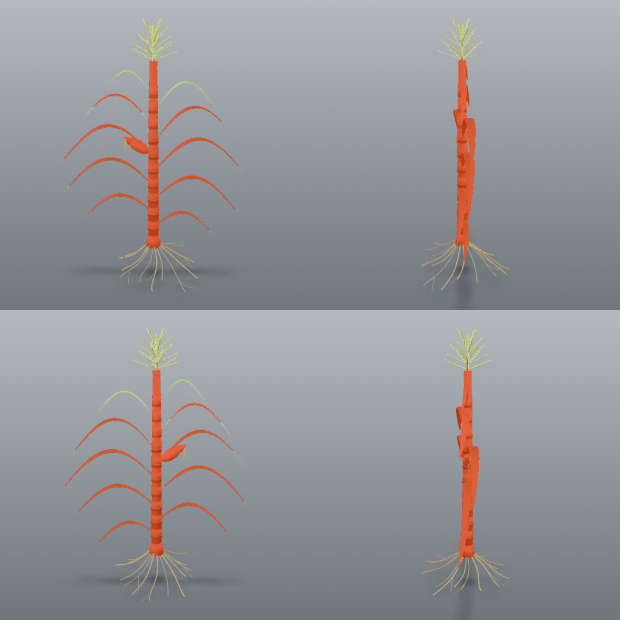 |
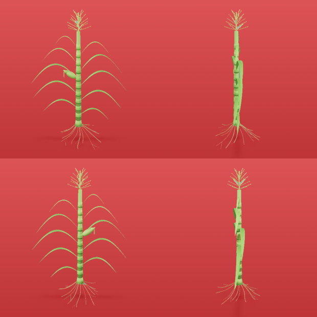 |
Mask covers 3.1% of the frame, 9 components. area=32427 |
Mask covers 96.1% — it is the background. area=1007829 |
The failure on the right is what this server exists to prevent. Without the picture, both runs return seventeen traits with correct units and entirely believable magnitudes. The one on the right is measuring the wall behind the plants.
segment() returns the overlay and diagnostics but no traits. measure() requires the
session_id that segment() mints. You cannot get a number without first being handed the
image it came from.
That is not a style preference. Measured on real images with PlantCV 4.11.3:
| failure | what you get without the overlay |
|---|---|
| four-view render, whole-image ROI | 17 plausible traits describing four merged plants |
| plant clipped by the frame | size traits that are silently lower bounds |
| empty mask | 17 traits of zeros, with PlantCV reporting in_bounds=True |
All three produce correctly-united, entirely believable numbers.
Install
pip install plantcv-mcp
Or from the repository, to track unreleased changes:
uv add git+https://github.com/musharna/plantcv-mcp
Or from a local checkout:
uv add /path/to/plantcv-mcp
Requires Python 3.11+. Installing pulls PlantCV and its scientific stack (scikit-image, dask, scipy), so the first install is not fast.
Configure your MCP client
The server speaks stdio. The console script installed by the package is
plantcv-mcp.
Claude Code
claude mcp add plantcv -- plantcv-mcp
Claude Desktop — add to claude_desktop_config.json:
{
  "mcpServers": {
    "plantcv": {
      "command": "plantcv-mcp"
    }
  }
}
If the executable is not on your PATH (common when it lives in a project
virtualenv), give the absolute path to it, or invoke it through uv:
{
  "mcpServers": {
    "plantcv": {
      "command": "uv",
      "args": ["run", "--directory", "/path/to/plantcv-mcp", "plantcv-mcp"]
    }
  }
}
Verify it is wired up by calling list_methods(), which reports the channels,
the methods, and the pinned PlantCV version.
Tools
| tool | returns |
|---|---|
suggest_segmentation(image_path, channel, method) |
contact sheets, and what each object_type would yield |
segment(image_path, channel, method, ...) |
overlay + diagnostics + warnings — no traits |
measure(session_id, analyses, px_per_mm, ...) |
traits, or a raised error on a degenerate mask |
calibrate_scale_from_marker(image_path, x, y, w, h, marker_length_mm) |
px_per_mm from a marker of known real size |
measure_images(image_paths, channel, method, ...) |
one recipe across many images; traits only where valid |
list_methods() |
channels, methods, object types, pinned PlantCV version |
Typical loop: suggest_segmentation → segment → look at the overlay → segment again
with a different channel, method or polarity if it is wrong → measure.
segment parameters
| parameter | default | what it does |
|---|---|---|
image_path |
required | image to read from the host filesystem |
channel |
required | one of l a b h s v — never guessed for you |
method |
required | one of otsu triangle mean gaussian |
object_type |
"dark" |
which side of the threshold is the plant. See below |
fill_size |
200 |
drops components smaller than this; can erase a small specimen |
ksize |
11 |
neighbourhood size, mean and gaussian only |
offset |
2 |
constant subtracted from the local mean, mean/gaussian only |
The segment() response for the image at the top of this page — verbatim, apart from a
shortened session_id and an elided warning message:
{
  "session_id": "9d2384c8-…",
  "channel": "a",
  "method": "otsu",
  "object_type": "dark",
  "fill_size": 200,
  "mask_fraction": 0.031,
  "component_count": 9,
  "major_object_count": 4,
  "largest_area": 8628,
  "overlay_scale": 1.0,
  "overlay_png_bytes": 748233,
  "warnings": [
    {
      "code": "multi_specimen",
      "message": "4 comparably-sized objects detected (areas: [8628, 7981, 7106, 6748]). …"
    }
  ]
}
The overlay arrives alongside this as a second content block, as an image.
Getting the polarity right
object_type decides which side of the threshold is the plant, and it is the easiest way to
get a confidently wrong answer — that is the right-hand image at the top of this page.
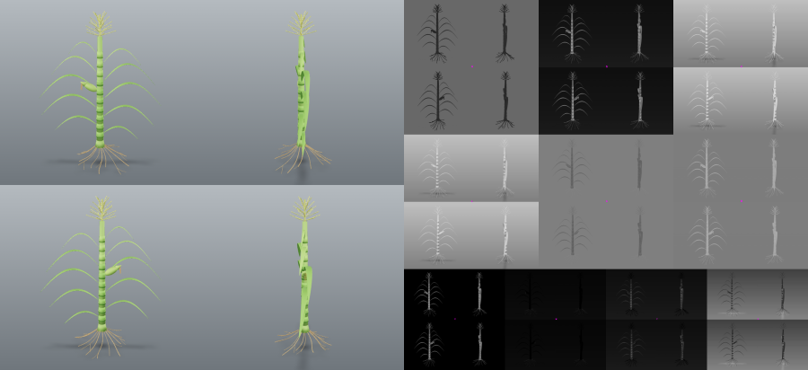
Two things guard against it. suggest_segmentation reports what both polarities yield on
your image before you commit, alongside a contact sheet of every colourspace:
And segment emits an implausible_coverage warning when the mask covers more than half the
frame. Neither refuses the measurement, because a macro shot of a single leaf legitimately
fills the frame — they make the choice visible rather than making it for you.
fill_size deletes any component smaller than itself, so a small specimen can vanish
entirely. When that happens segment reports fill_erased_mask and names the size to drop
below, rather than letting it look like a bad channel choice.
What it measures
One measure() call returns seventeen traits, each with a unit.
| group | traits |
|---|---|
| size | area, convex_hull_area, perimeter, total_edge_length, width, height, longest_path (pixels) |
| shape | solidity, convex_hull_vertices, ellipse_eccentricity (unitless) |
| ellipse fit | ellipse_major_axis, ellipse_minor_axis (pixels), ellipse_angle (degrees) |
| position | center_of_mass, ellipse_center (x, y) |
| PlantCV flags | in_bounds, object_in_frame |
The last two are PlantCV's own flags. They are passed through as information, never as
validity signals — on an all-zero mask PlantCV reports both as True while returning
seventeen zeros. They are bounds checks, not success checks.
Passing analyses=["size", "color"] adds hue, saturation and value statistics —
hue_circular_mean, hue_circular_std, hue_median (degrees), saturation_mean,
saturation_median, value_mean, value_median (percent). The three frequency histograms
that accompany them total 692 numbers, so they are withheld unless you ask for them with
include_histograms=true.
Real-world units
Traits are in pixels by default, and pixel sizes are not comparable between images shot at
different distances or zoom levels. Pass px_per_mm to measure() and spatial traits come
back in mm and mm2:
measure(session_id, px_per_mm=12.5)
  area    207.533 mm2     (32427 pixels)
  width    54.880 mm      (686 pixels)
Lengths divide by px_per_mm, areas by its square. That distinction is a hard-coded table
rather than something inferred from PlantCV's unit strings, because PlantCV labels both
area and width as "pixels" — scaling everything with that label linearly would leave
every area wrong by exactly a factor of px_per_mm, plausibly and silently. Positions
(center_of_mass, ellipse_center) stay in pixels, since a millimetre coordinate means
nothing without a defined origin.
If you have a marker of known real size in the frame — a coin, a printed disc — put a box around it and let the server measure it:
calibrate_scale_from_marker(image_path, x=100, y=100, w=100, h=100, marker_length_mm=20)
  -> px_per_mm 4.05, marker_length_px 81
marker_length_mm is the marker's longest real dimension. Check marker_length_px against
what you expect, because a wrong scale silently rescales every trait you measure afterwards.
The region is cropped before thresholding, so nothing outside your box can be selected;
PlantCV's own report_size_marker_area takes an ROI instead, and measured against a disc of
known 80 px diameter it returns 348 with a tight ROI — a silent 4.35× error. If the detected
object reaches the crop edge you get a marker_touches_crop_edge warning, which usually means
the polarity is wrong and the background was measured.
Colour correction
segment(..., color_correct=true) detects a Macbeth-style ColorChecker in the frame and
corrects to a standard reference, which is what makes colour traits comparable between images
shot under different lighting. measure() re-applies the same correction, so traits are always
measured on the pixels the mask was drawn on.
If no card is found this raises rather than quietly measuring the uncorrected image — returning colour traits that look corrected and are not would be the same kind of confident wrongness as an inverted mask.
Measuring many images
measure_images(image_paths, channel, method, ...) applies one fixed recipe across up to 200
images.
This is the one place the two-step discipline cannot hold literally: nobody reviews two hundred
overlays. So the overlay is replaced by the only honest substitute — every image runs the same
guards as segment(), and any image that trips a blocking guard comes back with no traits at
all, just a reason and an instruction to inspect it individually. Advisory warnings such as
multi_specimen are attached to the traits rather than suppressing them.
{
  "summary": {
    "submitted": 2,
    "measured": 1,
    "needs_review": 1,
    "review_paths": ["blank.png"]
  },
  "results": [
    {
      "image_path": "blank.png",
      "measured": false,
      "traits": null,
      "refused_because": "empty_mask — traits withheld because the mask probably does not describe the plant."
    }
  ]
}
Settle the recipe on one representative image with suggest_segmentation and segment first,
looking at the overlay, then apply it here. A batch never returns a number the server could not
validate — which is weaker than a human looking at a mask, and is stated plainly rather than
implied.
Security and trust boundary
This server reads image files anywhere on the host filesystem, and returns them to the model as images.
suggest_segmentation and segment take an image_path and pass it straight to
PlantCV's reader. There is no directory allow-list and no sandbox. Any path the
model asks for — that the operating-system user running the server can read — will
be decoded and returned as a base64 image in the model's context.
Practical consequences:
- Treat it like any other local filesystem MCP server. Run it as a user whose read access you are comfortable exposing to the model driving it.
- A prompt-injected or adversarial model can use it to view arbitrary image files on the machine. Non-image files fail to decode and raise, but the error message discloses whether the path exists.
- Do not run it as root, and do not expose it to untrusted input on a machine holding sensitive imagery.
Restricting reads to a configured root directory is a candidate for a future release; it is deliberately not implemented today, and this section exists so that is a decision you make rather than a surprise you discover.
Limitations
Phase 1 is single-ROI: measure() uses the whole image as its region of
interest, which is why the multi-specimen warning can only advise rather than
correct. Multi-plant grids, morphology traits (leaf angles, stem, skeleton) and
iterative mask refinement are phase 2.
Sessions are in-memory and capped (8 by default, LRU-evicted). They do not survive a server restart.
Attribution and licensing
This project is MIT licensed. It depends on PlantCV, which is licensed under the Mozilla Public License 2.0. No PlantCV source is vendored or redistributed here — it is an ordinary runtime dependency — so the MIT license applies to this project's own files. See NOTICE for the full statement.
More
- CHANGELOG.md — what changed, and why
- docs/MUTATION-CHECKS.md — every guard disabled on purpose, and the test that went red for it. A guard whose test passes with the guard removed is not a test.
Images on this page are rendered from tests/fixtures/multi_specimen.png, an original render
by the author, and regenerate from committed code.
Release history Release notifications | RSS feed


Download files
Download the file for your platform. If you're not sure which to choose, learn more about installing packages.
Source Distribution
Built Distribution
Filter files by name, interpreter, ABI, and platform.
If you're not sure about the file name format, learn more about wheel file names.
Copy a direct link to the current filters
File details
Details for the file plantcv_mcp-0.3.0.tar.gz.
File metadata
- Download URL: plantcv_mcp-0.3.0.tar.gz
- Upload date:
- Size: 241.1 kB
- Tags: Source
- Uploaded using Trusted Publishing? No
- Uploaded via: twine/6.2.0 CPython/3.13.2
File hashes
| Algorithm | Hash digest | |
|---|---|---|
| SHA256 |
401bb1e67ac062d7636d481af61def1d1cd8c182892592393d47a0551d26cc16
|
|
| MD5 |
c8e54224e02386058264cf091de2163e
|
|
| BLAKE2b-256 |
083382710fcd86983f009c0861438fa7393e6f084390c638a719417921de38c0
|
File details
Details for the file plantcv_mcp-0.3.0-py3-none-any.whl.
File metadata
- Download URL: plantcv_mcp-0.3.0-py3-none-any.whl
- Upload date:
- Size: 33.5 kB
- Tags: Python 3
- Uploaded using Trusted Publishing? No
- Uploaded via: twine/6.2.0 CPython/3.13.2
File hashes
| Algorithm | Hash digest | |
|---|---|---|
| SHA256 |
fb39d3df44c886c9f592df13ed04b293b5fd0e1654c17ddd1a2f01254b1af4d3
|
|
| MD5 |
180d9913b381954c205e1a4a404f7dd3
|
|
| BLAKE2b-256 |
06d7e4457882405274717955c4bab00d68bf1e3506e366f36e6c9aacaf6534e1
|






