
plot3
ggplot2 for Python, plus what ggplot2 can't do: interactive 3D, animated data, and plots typed straight from an equation. Figures render with WebGL in the notebook and save as journal-ready PNG, SVG, or PDF.
 |
 |
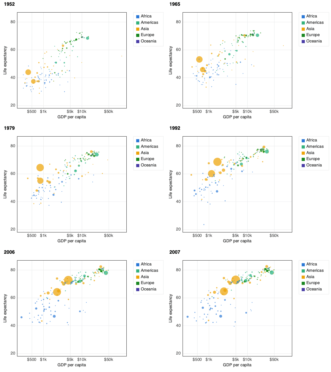
+ transition_time("year"): gapminder in one line |
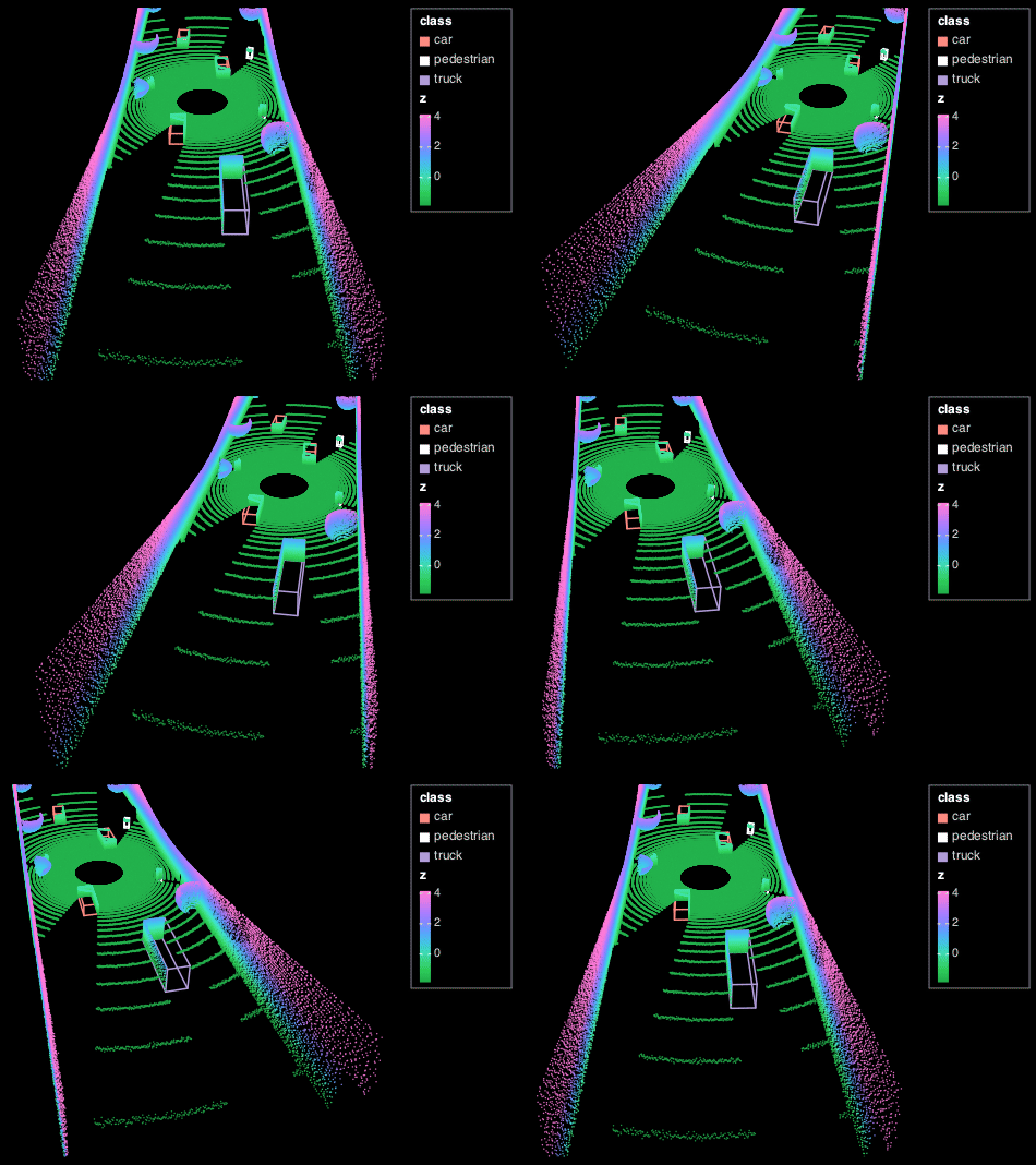
geom_point3d() + geom_box3d(): a 220k-point lidar sweep with detection boxes |
 |
 |
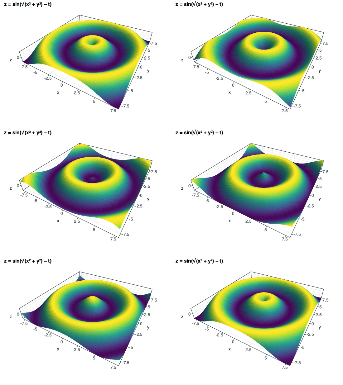
geom_function("z = sin(sqrt(x^2 + y^2) - t)") + transition_time(t=(0, 6.28)) |
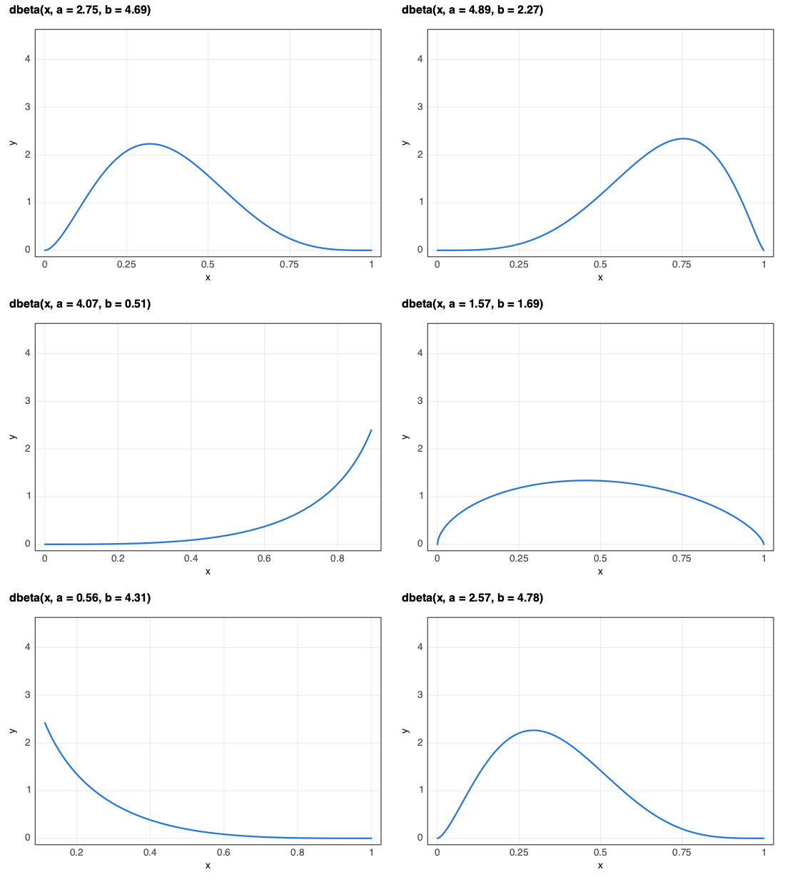
geom_function("y = dbeta(x, a, b)") + slider(a=…, b=…) |
pip install "plot3[jupyter,export]"
Contents: Plot an equation · Animate your data · 3D and point clouds · One figure, two outputs · It's ggplot2 · Notebooks, SolveIt, CRAFT · Install · Full reference
Plot an equation
Write the maths as you would on paper. geom_function works out whether
it's a curve, an implicit shape, a region, or a 3D surface, and picks a
sensible window.
from plot3 import *

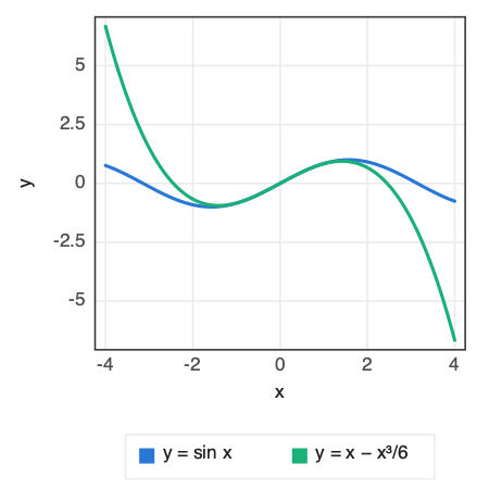
(ggplot() + geom_function("y = sin(x)", xlim=(-4, 4))                        # a function and
 + geom_function("y = x - x^3/6", xlim=(-4, 4)))                            # its Taylor polynomial
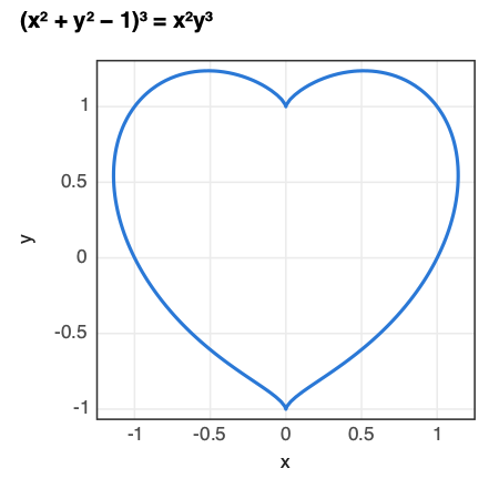
ggplot() + geom_function("(x^2 + y^2 - 1)^3 = x^2 y^3")                     # implicit: a heart
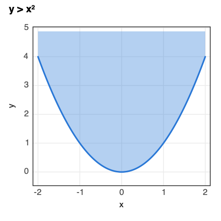
ggplot() + geom_function("y > x^2", xlim=(-2, 2))                           # shaded region
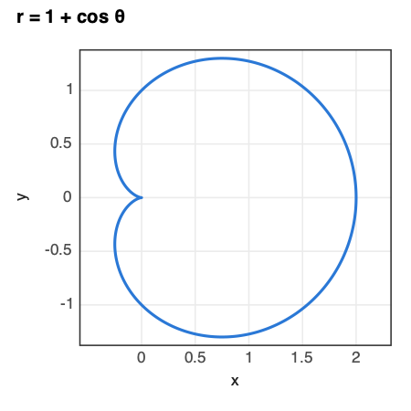
ggplot() + geom_function("r = 1 + cos(theta)") + coord_polar()              # polar cardioid
ggplot() + geom_function(r"z = \frac{\sin\sqrt{x^2+y^2}}{\sqrt{x^2+y^2}}",  # LaTeX in, 3D sombrero out
                         xlim=(-10, 10), ylim=(-10, 10))
ggplot() + geom_vector_field("dx = y, dy = -sin(x) - 0.3y",                # a damped pendulum's
                          xlim=(-6, 6), ylim=(-3, 3), stream=True)          # phase portrait
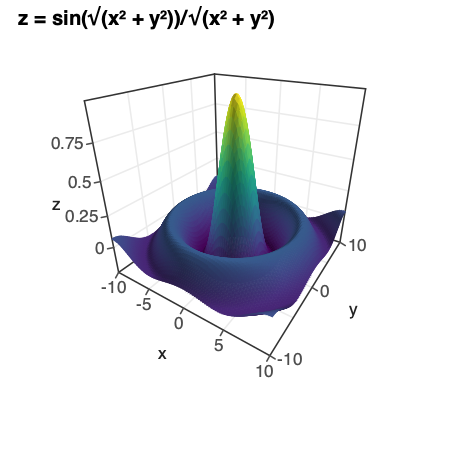
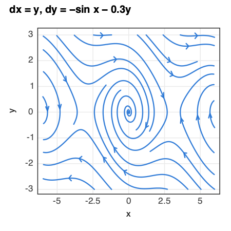
Probability and calculus, with the answer printed. No SciPy needed:
inf = float("inf")
ggplot() + geom_function("y = dbeta(x, 2, 5)") + area(0.2, 0.5)          # labels P(0.2 ≤ X ≤ 0.5) = 0.546
ggplot() + geom_function("y = dnorm(x)") + area(-inf, -1.96) + area(1.96, inf)
ggplot() + geom_function("y = x^3 - 3x") + tangent(at=1) + derivative()
Turn any coefficient into a slider or an animation:
ggplot() + geom_function("y = dbeta(x, a, b)") + slider(a=(0.5, 5), b=(0.5, 5))
ggplot() + geom_function("y = sin(x - t)") + transition_time(t=(0, 6.28))   # travelling wave
Equations mix freely with data:
ggplot(df, aes(x="dose", y="response")) + geom_point() + geom_function("y = 2 + 0.6x").
^ is power and 2x means 2*x. All functions, densities, and rules are in
the reference.
Animate your data
gganimate's grammar: add a transition and the plot plays. The viewer interpolates between frames in the browser, with play, pause, scrubbing, speed control, and one-click video export.
import pandas as pd
gapminder = pd.read_csv("https://raw.githubusercontent.com/kirenz/datasets/master/gapminder.csv")

(ggplot(gapminder, aes(x="gdpPercap", y="lifeExp", size="pop", colour="continent", group="country"))
 + geom_point(alpha=0.7)
 + scale_x_log10()
 + transition_time("year")
 + labs(title="{frame_time}", x="GDP per capita", y="Life expectancy"))
{frame_time} in the title shows the current year as it plays.
transition_states("phase") steps through categories instead of time.
Run this without downloading anything (made-up gapminder-shaped data)
import pandas as pd

countries = {"Brazil": "Americas", "China": "Asia", "Egypt": "Africa",
             "France": "Europe", "India": "Asia", "Mexico": "Americas"}
gapminder = pd.DataFrame([
    {"country": country, "continent": continent, "year": year,
     "gdpPercap": 800 * (1.03 + 0.01 * i) ** (year - 1952),
     "lifeExp": 45 + 0.35 * (year - 1952) + 2 * i,
     "pop": 2e7 * (1.02 + 0.002 * i) ** (year - 1952)}
    for i, (country, continent) in enumerate(countries.items())
    for year in range(1952, 2008, 5)
])

(ggplot(gapminder, aes(x="gdpPercap", y="lifeExp", size="pop", colour="continent", group="country"))
 + geom_point() + scale_x_log10() + transition_time("year") + labs(title="{frame_time}"))
3D and point clouds
Map z and the plot becomes a 3D scene you can orbit, zoom, and hover.
Hundreds of thousands of points stay smooth because they're drawn on the
GPU.
import numpy as np

rng = np.random.default_rng(0)
arm = rng.integers(0, 2, 20_000)
r = rng.gamma(2, 1.2, 20_000)
theta = r * 0.9 + arm * np.pi + rng.normal(0, 0.25, 20_000)
galaxy = pd.DataFrame({"x": r * np.cos(theta), "y": r * np.sin(theta),
                       "z": rng.normal(0, 0.15, 20_000), "r": r})

(ggplot(galaxy, aes(x="x", y="y", z="z", colour="r"))
 + geom_point3d(size=0.01) + scale_colour_viridis_c(option="magma")
 + coord_3d(elev=40) + theme_lidar() + guides(colour="none"))

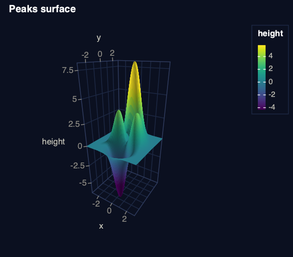
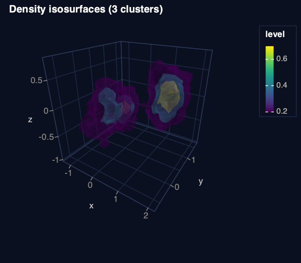
Surfaces, isosurfaces, and self-driving scenes use the same grammar:
ggplot(grid, aes(x="x", y="y", z="height", fill="height")) + geom_surface()
ggplot(points, aes(x="x", y="y", z="z")) + geom_isosurface(levels=[0.2, 0.5, 0.8])

(ggplot(sweep, aes(x="x", y="y", z="z"))                 # a nuScenes / KITTI lidar sweep
 + geom_point3d()                                         # coloured by height, as lidar viewers do
 + geom_box3d(aes(length="l", width="w", height="h", angle="yaw", colour="class"), data=boxes)
 + coord_3d(azim=180, elev=28, zoom=1.6)                 # chase camera behind the car
 + theme_lidar())
read_bin("scan.pcd.bin") loads nuScenes-style point clouds, and NumPy
arrays work by column position: aes(x=0, y=1, z=2, colour=3). Camera,
aspect, and point-budget options are in the
reference under coord_3d.
One figure, two outputs
The same object is an interactive figure in the notebook and a publication
figure on disk, with real fonts, correct DPI metadata, and theme_bw by
default.
ggsave("fig1.pdf", p, width=3.5, height=2.6, units="in")         # vector, one journal column
ggsave("fig1.png", p, width=7, height=4.5, units="in", dpi=300)   # two columns
ggsave("fig1.html", p)                                            # interactive page to share
It's ggplot2
If you know ggplot2, you already know plot3: + layers, aes(), geoms,
stats, scales, facets, themes, labs(), and patchwork's | and /, with
ggplot2's names and defaults.
rng = np.random.default_rng(1)
trial = pd.DataFrame({"arm": rng.choice(["placebo", "low", "high"], 150),
                      "dose": rng.uniform(0, 10, 150)})
trial["response"] = 2 + 0.6 * trial.dose + 1.5 * (trial.arm == "high") + rng.normal(0, 1.2, 150)

a = (ggplot(trial, aes(x="dose", y="response", colour="arm"))
     + geom_point(alpha=0.7) + geom_smooth(method="lm"))
b = (ggplot(trial, aes(x="arm", y="response", fill="arm"))
     + geom_violin() + geom_jitter(width=0.1, height=0) + theme(legend_position="none"))
fig = (a | b) + plot_annotation(title="Response by dose and arm", tag_levels="A")

Everything else you'd expect is there, including histograms, densities,
boxplots, bar positions, stat_summary, error bars, heatmaps, hexbins, 2D
densities, facet_wrap / facet_grid, Brewer, viridis, and Okabe–Ito
scales, date axes, theme() with element_*(), and coord_flip /
coord_polar. See the full reference for what
plot3 supports and how it differs from ggplot2, or use the
ggplot2 docs directly; the
names match.
In notebooks, bare column names work as in R: aes(x=dose, y=response).
Notebooks, SolveIt, and CRAFT
- Jupyter / SolveIt: bare column names and backticks work in
aes(),facet_wrap(), andfacet_grid()(aes(x=First Name)). Toggle withenable_r_style()/disable_r_style()..pyfiles keep quoted strings. - SolveIt draws figures inline and hides their HTML from the model's
context (
autohide(False)to opt out). - VS Code notebooks block WebGL in output cells, so plot3 opens figures
in your browser (
PLOT3_DISPLAY=browser|iframeto force a mode). The page is written to.plot3_preview/latest.htmlin the notebook's folder, or to the system temp folder when that folder is read-only. - CRAFT /
%gpu: the sameggplot(...)code runs on the remote kernel; stats run where the data lives and only a compact payload comes back.
%run /path/to/plot3/plot3.py        # loads plot3 locally and seeds the GPU kernel
%plot3 df x=wt y=mpg color=cyl       # optional shortcut magic
Install
pip install "plot3[jupyter,export]"
Python 3.10 or newer; NumPy and pandas are the only required packages.
| Extra | Adds |
|---|---|
export |
cairosvg: PNG with real fonts and PDF. Needs the Cairo C library (brew install cairo, apt install libcairo2). SVG needs nothing. |
fast |
contourpy: faster implicit-curve contours (matplotlib users have it) |
jupyter |
IPython integration (bare column names, %plot3) |
polars |
Polars tables |
The latest unreleased code installs from GitHub with
pip install "plot3[jupyter,export] @ git+https://github.com/rleyvasal/plot3".
Development
git clone https://github.com/rleyvasal/plot3 && cd plot3
python3 -m venv .venv && source .venv/bin/activate
pip install -e ".[dev,jupyter,export]"
pytest -q                       # includes every example in this README and docs/reference.md
python examples/showcase_2d.py  # 2D gallery in the browser
python examples/showcase_3d.py  # 3D gallery
The code is in plot3/: geoms.py (grammar objects), scaling.py
(scale functions), build.py (stats to a figure spec), stat2d.py and
flip.py (statistical layers), static.py (PNG/SVG/PDF), viewer.py (the
WebGL viewer), expr.py / function.py / calculus.py (formulas),
compose.py (multi-panel figures). See CHANGELOG.md for
changes between versions.
License
MIT. See LICENSE.
1 maintainer

Metadata
1 maintainer
Release files for plot3 0.5.1
For a detailed explanation of source distributions (sdists) and built distributions (wheels), please see the package formats documentation.
Source distribution (sdist)
| File | Size | Uploaded | Provenance | Actions |
|---|---|---|---|---|
| plot3-0.5.1.tar.gz | 377.1 kB | With provenance | Details for plot3-0.5.1.tar.gz |
Built distribution (wheel)
| File | Interpreter | ABI | Platform | Actions Reset |
|---|---|---|---|---|
| plot3-0.5.1-py3-none-any.whl | Python 3 | none | any | Details for plot3-0.5.1-py3-none-any.whl |
Total release size: 680.5 kB
Release files / plot3-0.5.1.tar.gz
| Download URL | plot3-0.5.1.tar.gz |
|---|---|
| Size | 377.1 kB |
| Tags | Source |
|
SHA-256 checksum How to use checksums |
ce9bcd6b55bc0164663a01b3d29f5e5b70c59a94b587978cff013a776f41b59c
|
|
BLAKE2b-256 checksum How to use checksums |
10f557c6719cb154d787b2e147e0ee3e6ffe5a9230a9a07182479e4d9e7a732a
|
| Upload date | |
|
Uploaded using Trusted Publishing? What is trusted publishing? |
Yes |
| Uploaded via |
twine/7.0.0 CPython/3.13.14
|
Provenance
Provenance describes where a file came from. On PyPI, provenance is shared via attestations, which provide a verifiable record of the build or publishing details. View details, limitations and caveats.


PyPI Publish Attestation
PyPI verified that this artifact, at this checksum, originated from the publisher listed below.
Signed by GitHub Actions, verified by PyPI on Oct 10, 2026.
Transparency logRelease files / plot3-0.5.1-py3-none-any.whl
| Download URL | plot3-0.5.1-py3-none-any.whl |
|---|---|
| Size | 303.4 kB |
| Tags | Python 3 |
|
SHA-256 checksum How to use checksums |
13fe86be9bcea35c553e724c67203c90749f35f47f184f4f2c7bad2e1c53f7aa
|
|
BLAKE2b-256 checksum How to use checksums |
597eb05fcc1139ea618397be18e51f06c7ebe313d4478cb6964ca3a7e03e8a17
|
| Upload date | |
|
Uploaded using Trusted Publishing? What is trusted publishing? |
Yes |
| Uploaded via |
twine/7.0.0 CPython/3.13.14
|
Provenance
Provenance describes where a file came from. On PyPI, provenance is shared via attestations, which provide a verifiable record of the build or publishing details. View details, limitations and caveats.
PyPI Publish Attestation
PyPI verified that this artifact, at this checksum, originated from the publisher listed below.
Signed by GitHub Actions, verified by PyPI on Oct 10, 2026.
Transparency logSecurity for plot3 0.5.1
Provenance
Provenance describes where a file came from. On PyPI, provenance is shared via attestations, which provide a verifiable record of the build or publishing details. View details, limitations and caveats.
Full provenance
Both files in this release have been uploaded with provenance metadata.
Attestation for plot3-0.5.1.tar.gz
PyPI Publish Attestation
PyPI verified that this artifact, at this checksum, originated from the publisher listed below.
Signed by GitHub Actions, verified by PyPI on Oct 10, 2026.
Transparency logA note on package security
PyPI is a repository for distributing packages, not a service for auditing them. While third-party security researchers and our staff do their best to detect and remove malicious packages, PyPI cannot guarantee the quality, security or suitability of any given package.
To learn more about protecting yourself from malicious actors, visit our package security documentation.














