Matplotlib/seaborn style presets matching scientific journal requirements, with validation, export safety, and preview capabilities.
Verified details
These details have been verified by PyPIProject links
GitHub Statistics
Maintainers

Project description
plotstyle
Matplotlib figures formatted for journal submission, automatically.


PlotStyle makes it easy to produce Matplotlib figures that meet the exact typographic, dimensional, and export requirements of major academic journals. It integrates with Seaborn, with more integrations planned.
Each journal is represented as a named preset: a complete set of font, column width, colour, and export settings sourced from the journal's official author guidelines.
- Apply correct font sizes, column widths, and DPI for all supported journals with one call
- Validate figures against journal requirements before you submit
- Export in all required file formats at once
- Simulate colorblind and grayscale rendering to catch accessibility issues early
- Use overlays to adapt style for notebooks, presentations, or custom palettes
- Compare two journal presets side by side with
plotstyle.diff()
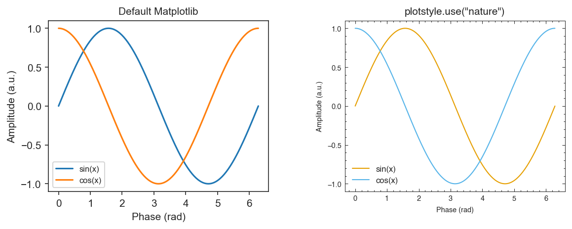
Left: default Matplotlib. Right: plotstyle.use("nature") - Nature single-column width (89 mm), Helvetica, 7 pt, 300 DPI. Same data, different style.
Table of Contents
Installation
Requires Python 3.10+ and Matplotlib >= 3.9.
pip install plotstyle
If you are unsure which extras to install, use [all]:
pip install "plotstyle[all]"
Or install only what you need:
pip install "plotstyle[seaborn]"    # seaborn integration
pip install "plotstyle[fonttools]"  # better PDF font subsetting
If fonts look wrong after installation, run plotstyle fonts --journal <name> to see which fonts are required, which are installed, and which one was selected as a fallback. If no required fonts are installed, install one from the listed names and then rebuild matplotlib's font cache:
python -c "from matplotlib.font_manager import _load_fontmanager; _load_fontmanager(try_read_cache=False)"
Quick Start
The with block is the recommended pattern. Matplotlib's rcParams are restored automatically when it exits, even if an exception occurs.
import numpy as np
import plotstyle
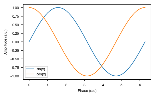
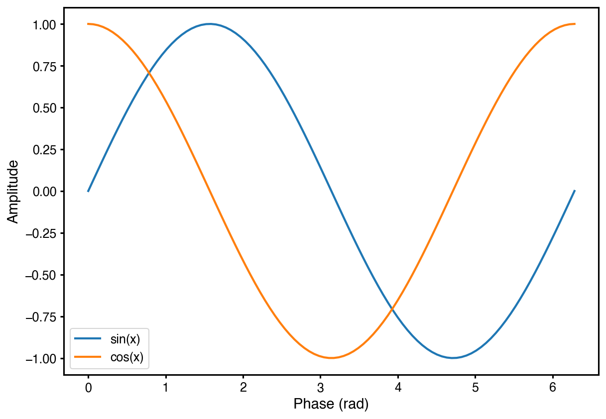
with plotstyle.use("nature") as style:
fig, ax = style.figure(columns=1) # sized to Nature's single-column width (89 mm)
x = np.linspace(0, 2 * np.pi, 200)
ax.plot(x, np.sin(x), label="sin(x)")
ax.plot(x, np.cos(x), label="cos(x)")
ax.set_xlabel("Phase (rad)")
ax.set_ylabel("Amplitude (a.u.)")
ax.legend()
style.savefig(fig, "figure.pdf") # 300 DPI minimum, TrueType fonts embedded
Pass
latex="auto"toplotstyle.use()to enable LaTeX rendering when a LaTeX binary is on PATH, falling back to MathText otherwise. Uselatex=Trueto force LaTeX, orlatex=False(default) to always use MathText.
Outside a
withblock,plotstyle.savefig(fig, "figure.pdf", journal="nature")saves with the same DPI and font settings without needing the context manager.
Examples
This section covers multi-panel figures, color palettes, overlays, accessibility checks, validation, and submission export.
Multi-panel figures
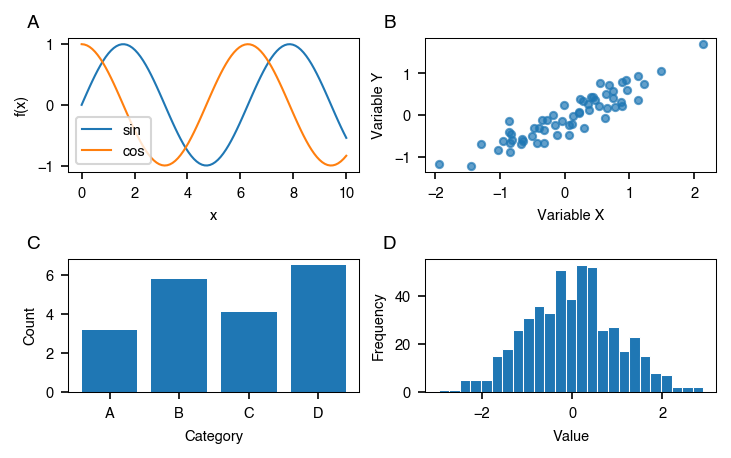
style.subplots() works like plt.subplots() but sizes the figure to the journal preset and adds panel labels automatically. All built-in journal presets use bold lowercase labels (a, b, c, ...). The label style is driven by each preset's panel_label_case field and can be lower, upper, parens_lower, parens_upper, sentence, or title.
import numpy as np
import plotstyle

rng = np.random.default_rng(42)

with plotstyle.use("science") as style:
    fig, axes = style.subplots(nrows=2, ncols=2, columns=2)

    x = np.linspace(0, 10, 100)
    axes[0, 0].plot(x, np.sin(x), label="sin")
    axes[0, 0].plot(x, np.cos(x), label="cos")
    axes[0, 0].set_xlabel("x")
    axes[0, 0].set_ylabel("f(x)")
    axes[0, 0].legend()

    xs = rng.normal(0, 1, 60)
    ys = 0.7 * xs + rng.normal(0, 0.3, 60)
    axes[0, 1].scatter(xs, ys, s=12, alpha=0.7)
    axes[0, 1].set_xlabel("Variable X")
    axes[0, 1].set_ylabel("Variable Y")

    axes[1, 0].bar(["A", "B", "C", "D"], [3.2, 5.8, 4.1, 6.5])
    axes[1, 0].set_xlabel("Category")
    axes[1, 0].set_ylabel("Count")

    axes[1, 1].hist(rng.normal(0, 1, 500), bins=25, edgecolor="white", linewidth=0.5)
    axes[1, 1].set_xlabel("Value")
    axes[1, 1].set_ylabel("Frequency")

    style.savefig(fig, "multi_panel.pdf")
axesis always a 2-D NumPy array. Useaxes[0, 0]to access a single panel oraxes.flatto iterate. Passpanels=Falseto suppress the automatic labels.
Pass
aspect=<ratio>tostyle.figure()orstyle.subplots()to override the default golden ratio width-to-height ratio.
Color palettes
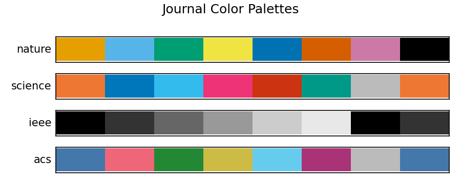
Each journal has a recommended colorblind-safe palette. plotstyle.palette() returns hex color strings, cycling if you need more than the palette length.
import plotstyle

colors = plotstyle.palette("nature", n=4)
print(colors)
# ['#E69F00', '#56B4E9', '#009E73', '#F0E442']

plotstyle.list_palettes()   # list all available palette names
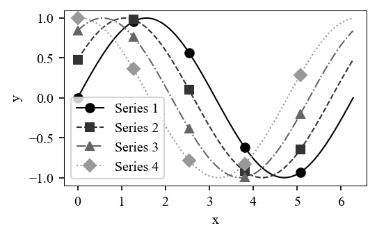
Pass with_markers=True to get (color, linestyle, marker) tuples, useful for journals like IEEE that print in grayscale:
import numpy as np
import plotstyle

x = np.linspace(0, 2 * np.pi, 100)
curves = [np.sin(x + i * 0.5) for i in range(4)]

with plotstyle.use("ieee") as style:
    fig, ax = style.figure(columns=1)
    styled = plotstyle.palette("ieee", n=4, with_markers=True)
    for i, (color, ls, marker) in enumerate(styled):
        ax.plot(x, curves[i], color=color, linestyle=ls, marker=marker,
                markevery=20, linewidth=0.8, markersize=3, label=f"Series {i + 1}")
    ax.set_xlabel("x")
    ax.set_ylabel("y")
    ax.legend(fontsize=7)
    style.savefig(fig, "ieee_markers.pdf")
# styled: one (color, linestyle, marker) tuple per series:
[('#000000', '-', 'o'), ('#333333', '--', 's'), ('#666666', '-.', '^'), ('#999999', ':', 'D')]
To apply a named palette directly to a specific axes or globally, use plotstyle.apply_palette():
from plotstyle.color.palettes import apply_palette

apply_palette("okabe-ito", ax=ax)   # sets the colour cycle on this axes only
apply_palette("tol-bright")         # sets it globally for all subsequently created axes
Overlays
Overlays are additive patches that layer on top of a journal preset. They let you adjust one aspect of a figure (the colour palette, the context, the chart type) without changing the base journal settings.
| Category | Purpose | Examples |
|---|---|---|
color |
Swap the colour cycle | okabe-ito, conservative-colorblind, tol-bright, tol-high-contrast, tol-light, tol-muted, tol-vibrant, tol-rainbow-{1..23}, safe-grayscale |
context |
Adjust scale for the medium | notebook, presentation, minimal, high-vis |
rendering |
Control LaTeX and grid rendering | no-latex, grid, latex-sans, pgf, si-units |
plot-type |
Optimise for a chart type | bar, scatter |
script |
Non-Latin font support | cjk-simplified, cjk-traditional, cjk-japanese, cjk-korean, russian, turkish |
tol-vibrantis the default colour cycle for thesciencepreset. Use it as an overlay to apply the same palette to a different journal.
Pass overlay names in the same list as the journal preset:
import numpy as np
import plotstyle

x = np.linspace(0, 2 * np.pi, 100)

# Strip top/right spines for a clean editorial look
with plotstyle.use(["nature", "minimal"]) as style:
    fig, ax = style.figure(columns=1)
    for i in range(3):
        ax.plot(x, np.sin(x + i * 0.5), label=f"Series {i + 1}")
    ax.set_xlabel("Phase (rad)")
    ax.set_ylabel("Amplitude")
    ax.legend()
    style.savefig(fig, "minimal_figure.pdf")
import numpy as np
import matplotlib.pyplot as plt
import plotstyle

x = np.linspace(0, 2 * np.pi, 100)

# Larger figure and fonts for Jupyter notebooks
with plotstyle.use(["nature", "notebook"]) as style:
    fig, ax = plt.subplots()   # plt.subplots() picks up the notebook figsize
    ax.plot(x, np.sin(x), label="sin(x)")
    ax.plot(x, np.cos(x), label="cos(x)")
    ax.set_xlabel("Phase (rad)")
    ax.set_ylabel("Amplitude")
    ax.legend()
    style.savefig(fig, "notebook_figure.pdf")
import numpy as np
import plotstyle
x = np.linspace(0, 2 * np.pi, 100)
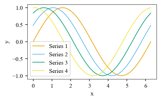
# Swap the colour cycle to a specific palette
with plotstyle.use(["ieee", "okabe-ito"]) as style:
fig, ax = style.figure(columns=1)
for i in range(4):
ax.plot(x, np.sin(x + i * 0.5), label=f"Series {i + 1}")
ax.set_xlabel("x")
ax.set_ylabel("y")
ax.legend()
style.savefig(fig, "okabe_ito_figure.pdf")
# List all available overlays
plotstyle.list_overlays()

# List overlays in a specific category
plotstyle.list_overlays(category="context")
# ['high-vis', 'minimal', 'notebook', 'presentation']
Overlay-only mode
Pass only overlay names to plotstyle.use() with no journal preset. PlotStyle adjusts the requested rcParams without applying any journal-specific fonts, sizes, or column widths. This is useful for blog posts, presentations, exploratory notebooks, or any context where journal compliance is not required.
import numpy as np
import matplotlib.pyplot as plt
import plotstyle

x = np.linspace(0, 2 * np.pi, 100)

with plotstyle.use(["notebook"]) as style:
    fig, ax = style.figure(columns=1)   # falls back to 6.4 in wide
    ax.plot(x, np.sin(x), label="sin(x)")
    ax.plot(x, np.cos(x), label="cos(x)")
    ax.set_xlabel("Phase (rad)")
    ax.set_ylabel("Amplitude")
    ax.legend()
    style.savefig(fig, "notebook_fig.pdf")
Combine multiple overlays in the same list. They are applied in declaration order and the last overlay wins on any rcParam conflict:
# Minimal axes (no top/right spines) with a subtle dashed grid
with plotstyle.use(["minimal", "grid"]) as style:
    fig, ax = style.figure()
    ax.plot(x, np.sin(x))
    ax.set_xlabel("x")
    ax.set_ylabel("y")
    style.savefig(fig, "minimal_grid.pdf")
For slides or posters, use the "presentation" overlay and create the figure with plt.subplots() so the overlay's larger figsize (10 x 7 in) is picked up:
with plotstyle.use(["presentation"]) as style:
    fig, ax = plt.subplots()   # uses the presentation figsize (10 x 7 in)
    ax.plot(x, np.sin(x), label="sin(x)")
    ax.set_xlabel("Phase (rad)")
    ax.set_ylabel("Amplitude")
    ax.legend()
    style.savefig(fig, "slide_fig.pdf")
In overlay-only mode,
style.palette(),style.validate(), andstyle.export_submission()raiseRuntimeErrorbecause they require a journal preset.style.savefig()accepts calls in any mode, but does not apply journal DPI or font-embedding settings without a preset.style.figure()always creates a figure.
style.figure()in overlay-only mode falls back to matplotlib's default width (6.4 in) and does not read anyfigure.figsizeset by an overlay. To pick up an overlay's figsize, useplt.subplots()instead (see thepresentationexample above).
Seaborn integration
Pass seaborn_compatible=True to plotstyle.use() to patch sns.set_theme so PlotStyle's rcParams are re-applied automatically after any seaborn theme change:
import seaborn as sns
import plotstyle

with plotstyle.use("nature", seaborn_compatible=True) as style:
    sns.set_theme(style="ticks")   # PlotStyle rcParams are re-applied automatically
    fig, ax = style.figure(columns=1)
    # ...
Colorblind and grayscale previews
Build a figure, then simulate how it looks under color vision deficiency or grayscale printing before you submit.
import numpy as np
import plotstyle
with plotstyle.use("nature") as style:
fig, ax = style.figure(columns=1)
x = np.linspace(0, 5, 80)
for i in range(4):
ax.plot(x, np.sin(x + i), linewidth=1.5, label=f"Series {i + 1}")
ax.set_xlabel("Time (s)")
ax.set_ylabel("Signal")
ax.legend()
# Simulate colour vision deficiency (deuteranopia, protanopia, tritanopia)
cvd_fig = plotstyle.preview_colorblind(fig)
cvd_fig.savefig("accessibility_colorblind.png", dpi=150, bbox_inches="tight")
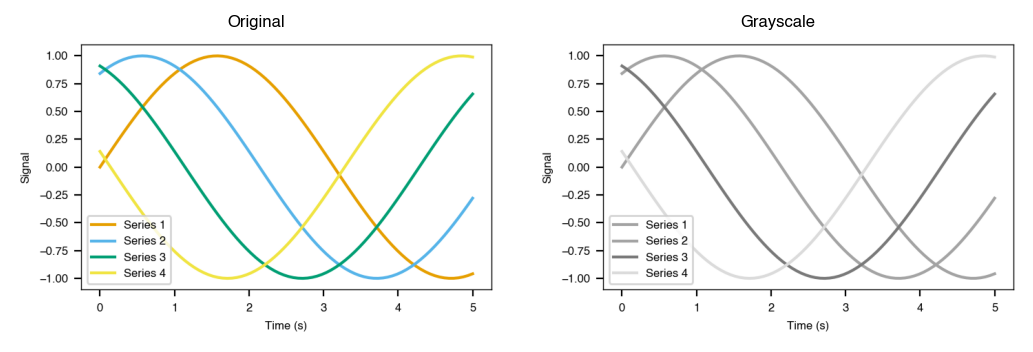
# Simulate grayscale print
gray_fig = plotstyle.preview_grayscale(fig)
gray_fig.savefig("accessibility_grayscale.png", dpi=150, bbox_inches="tight")
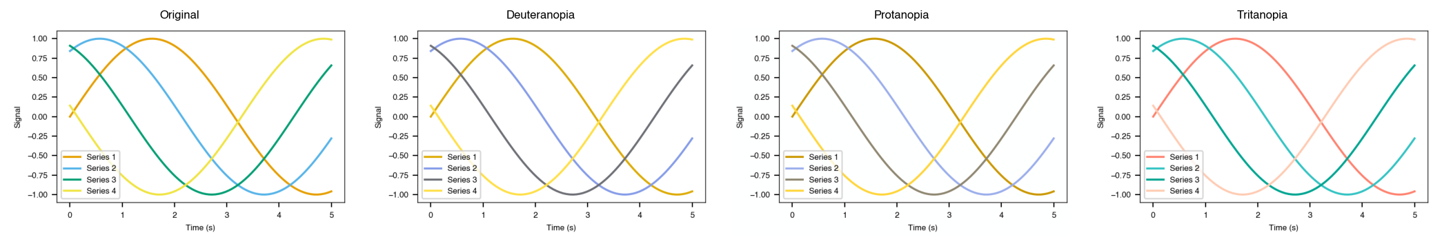
By default,
preview_colorblindsimulates deuteranopia, protanopia, and tritanopia. Pass acvd_typeslist to limit the simulation to specific types:plotstyle.preview_colorblind(fig, cvd_types=[CVDType.DEUTERANOPIA])(importCVDTypefromplotstyle.color.accessibility).
To preview a figure at its exact physical column width on screen, use preview_print_size:
plotstyle.preview_print_size(fig, journal="nature")
A dimension annotation is added temporarily and removed after display.
Grayscale safety checks
This section covers a lower-level programmatic API for checking colour contrast ratios directly. Use preview_grayscale() for a visual check; use these functions when you need exact luminance values or need to validate programmatically.
rgb_to_luminance(r, g, b)returns the BT.709 luminance of a single color.luminance_delta(colors)returns pairwise luminance differences sorted ascending; the weakest pair is always first.is_grayscale_safe(colors, threshold)returnsTrueonly when every pair meets the minimum delta.
from plotstyle.color.grayscale import luminance_delta, is_grayscale_safe
import plotstyle

# Pairwise deltas for a palette
colors = plotstyle.palette("nature", n=4)
deltas = luminance_delta(colors)
for i, j, delta in deltas:
    status = "pass" if delta >= 0.10 else "fail"
    print(f"[{status}] Color {i} vs Color {j}: delta = {delta:.4f}")

# Pass/fail check
safe = is_grayscale_safe(colors, threshold=0.10)
print(f"Grayscale safe: {safe}")
[fail] Color 0 vs Color 1: delta = 0.0048
[pass] Color 0 vs Color 2: delta = 0.1620
[pass] Color 1 vs Color 2: delta = 0.1668
[pass] Color 1 vs Color 3: delta = 0.2157
[pass] Color 0 vs Color 3: delta = 0.2205
[pass] Color 2 vs Color 3: delta = 0.3825
Grayscale safe: False
IEEE is the only built-in journal whose default palette (safe_grayscale) is designed for black-and-white printing. Most colorblind-safe palettes distinguish colors by hue and are not automatically safe in grayscale.
Validation and submission export
Validate a figure against the journal's requirements, then export in all required formats at once.
import numpy as np
import plotstyle

x = np.linspace(0, 2 * np.pi, 100)

with plotstyle.use("nature") as style:
    fig, ax = style.figure(columns=1)
    ax.plot(x, np.sin(x), label="sin(x)")
    ax.set_xlabel("Phase (rad)")
    ax.set_ylabel("Amplitude")
    ax.legend()

    report = plotstyle.validate(fig, journal="nature")
    print(report)
    print(report.passed)    # True
    print(report.failures)  # list of failed CheckResult objects; empty when all pass
    print(report.warnings)  # list of CheckResult objects with WARN status
    print(report.to_dict()) # JSON-serialisable dict
┌──────────────────────────────────────────────────────┐
│         PlotStyle Validation Report: Nature          │
├──────────┬───────────────────────────────────────────┤
│ ✓ PASS   │ Figure width 89.0mm matches single colu...│
│ ✓ PASS   │ Figure height 55.0mm is within the Natu...│
│ ✓ PASS   │ pdf.fonttype = 42 (TrueType fonts will ...│
│ ✓ PASS   │ ps.fonttype = 42 (TrueType fonts will b...│
│ ✓ PASS   │ savefig.dpi = 300.0 meets the Nature mi...│
│ ✓ PASS   │ All plotted lines and spines meet the N...│
│ ✓ PASS   │ All text elements are within the Nature...│
└──────────┴───────────────────────────────────────────┘
7/7 checks passed, 0 warning(s), 0 failure(s)

passed: True
When called outside plotstyle.use(), checks will fail and each failure.message and failure.fix_suggestion tells you exactly what to correct. See 05_validation.py for the full failing-case example.
import numpy as np
import os
import plotstyle

os.makedirs("submission", exist_ok=True)

with plotstyle.use("ieee") as style:
    fig, ax = style.figure(columns=1)
    x = np.linspace(0, 2 * np.pi, 100)
    ax.plot(x, np.sin(x), label="sin(x)")
    ax.set_xlabel("Phase (rad)")
    ax.set_ylabel("Amplitude")
    ax.legend()

    paths = plotstyle.export_submission(
        fig,
        "figure1",
        journal="ieee",
        author_surname="Smith",     # IEEE prepends the surname prefix to filenames; ignored by other journals
        output_dir="submission/",
    )
    print(paths)
[PosixPath('submission/smith_figure1.tiff'),
 PosixPath('submission/smith_figure1.eps'),
 PosixPath('submission/smith_figure1.pdf'),
 PosixPath('submission/smith_figure1.png')]
Scenario: paper submission workflow
A complete end-to-end workflow combining journal comparison, figure creation, validation, and batch export.
Step 1: compare two journal presets before committing
import plotstyle

result = plotstyle.diff("nature", "science")
print(result)
Nature → Science
──────────────────────────────────────────────────
Column Width (single):  89.0mm → 86.4mm
Min Font Size:          5.0pt → 7.0pt
Colorblind Required:    No → Yes
...
str(result) prints all differing fields; the output above is abbreviated. len(result) returns the total number of differences; bool(result) is truthy when any field differs; result.to_dict() returns a JSON-serialisable dictionary.
Steps 2-4: create figures, validate, and export inside one style block
import numpy as np
import plotstyle

rng = np.random.default_rng(42)
time = np.linspace(0, 5, 80)

with plotstyle.use("nature") as style:
    colors = style.palette(n=4)

    # Step 2: create figures
    fig1, ax1 = style.figure(columns=1)
    signal = np.exp(-time / 3) * np.sin(2 * np.pi * time)
    ax1.plot(time, signal, color=colors[0], label="Signal")
    ax1.fill_between(time, signal - 0.1, signal + 0.1, alpha=0.3, color=colors[0])
    ax1.set_xlabel("Time (s)")
    ax1.set_ylabel("Amplitude (a.u.)")
    ax1.legend()

    fig2, axes = style.subplots(nrows=1, ncols=2, columns=2)
    xs = rng.normal(0, 1, 50)
    ys = 0.7 * xs + rng.normal(0, 0.3, 50)
    axes[0, 0].bar(["Control", "Treatment A", "Treatment B"], [1.0, 1.34, 0.87])
    axes[0, 1].scatter(xs, ys, color=colors[1], s=10, alpha=0.8)

    # Step 3: validate each figure
    for label, fig in [("fig1", fig1), ("fig2", fig2)]:
        report = style.validate(fig)
        print(f"{label}: {'PASS' if report.passed else 'FAIL'} ({len(report.checks)} checks)")

    # Step 4: export in all formats the journal requires
    for label, fig in [("fig1", fig1), ("fig2", fig2)]:
        paths = style.export_submission(fig, label, output_dir="submission/", quiet=True)
        print(f"{label}: {[p.name for p in paths]}")
fig1: PASS (7 checks)
fig2: PASS (7 checks)
fig1: ['fig1.eps', 'fig1.pdf']
fig2: ['fig2.eps', 'fig2.pdf']
Use
plotstyle.diff()to compare any two journal presets before starting. Usestyle.validate()inside thewithblock to catch problems before they reach the submission portal.
If the target journal changes after figures are already created, use plotstyle.migrate() to re-style them in place:
import plotstyle

# Re-style an existing figure for a different journal
plotstyle.migrate(fig1, from_journal="nature", to_journal="science")
plotstyle.savefig(fig1, "figure_science.pdf", journal="science")
migrate() resizes the figure to the target journal's column width, proportionally rescales all text, and emits warnings for font changes or DPI increases.
Supported Journals
| Key | Journal | Publisher |
|---|---|---|
acs |
ACS (JACS) | American Chemical Society |
acm |
ACM | Association for Computing Machinery |
cell |
Cell | Cell Press |
elsevier |
Elsevier | Elsevier |
ieee |
IEEE Transactions | IEEE |
nature |
Nature | Springer Nature |
plos |
PLOS ONE | Public Library of Science |
prl |
Physical Review Letters | American Physical Society |
science |
Science | AAAS |
springer |
Springer | Springer |
usenix |
USENIX | USENIX Association |
wiley |
Wiley | Wiley |
Run plotstyle info <journal> to see the source URL and last-verified date for any preset. Journal guidelines change over time; always confirm critical requirements against the journal's current author guidelines before submission.
Need another journal? See CONTRIBUTING.md for how to add a preset.
Use plotstyle.gallery("nature") to preview any journal's style across a line plot, scatter plot, bar chart, and histogram before writing plot code.
CLI
plotstyle --help                                        # show all commands
plotstyle list                                          # list all journal presets
plotstyle info <journal>                                # show preset details
plotstyle diff <journal_a> <journal_b>                  # compare two journal presets
plotstyle fonts --journal <journal>                     # check font availability for a journal
plotstyle fonts --overlay <overlay>                     # check font availability for a script overlay
plotstyle overlays [--category <category>]              # list available overlays
plotstyle overlay-info <overlay>                        # show overlay details
plotstyle validate <file.png|pdf> --journal <journal>   # check PDF font embedding
plotstyle export <file.png|pdf> --journal <journal>     # print a Python re-export snippet
plotstyle validate checks PDF files for Type 3 font embedding only. Full validation of dimensions, typography, and line weights requires a live Matplotlib figure: use plotstyle.validate(fig, journal=...) in Python.
plotstyle export does not create any output file. It prints a ready-to-run Python snippet that calls plotstyle.export_submission() with the specified settings. Re-export requires the original Matplotlib Figure object.
Full output examples are in the CLI reference.
Documentation
Full documentation is at plotstyle.readthedocs.io, including the installation guide, API reference, CLI reference, and FAQ. Working code examples are in the examples/ directory and interactive Jupyter notebooks are in examples/notebooks/.
Contributing
See CONTRIBUTING.md for development setup, adding journal presets, and pull request guidelines. All contributors are expected to follow the Code of Conduct.
To report a security vulnerability, use GitHub's private vulnerability reporting rather than opening a public issue. See SECURITY.md for scope, timeline, and disclosure guidelines.
If PlotStyle helps your research, a citation is appreciated. Use the "Cite this repository" button on the GitHub sidebar to get a ready-to-use APA or BibTeX entry. It reads from CITATION.cff and is always up to date.
License
MIT © 2026 Rahul Kaushal
Project details
Verified details
These details have been verified by PyPIProject links
GitHub Statistics
Maintainers
Release history Release notifications | RSS feed


Download files
Download the file for your platform. If you're not sure which to choose, learn more about installing packages.
Source Distribution
Built Distribution
Filter files by name, interpreter, ABI, and platform.
If you're not sure about the file name format, learn more about wheel file names.
Copy a direct link to the current filters
File details
Details for the file plotstyle-1.2.4.tar.gz.
File metadata
- Download URL: plotstyle-1.2.4.tar.gz
- Upload date:
- Size: 231.2 kB
- Tags: Source
- Uploaded using Trusted Publishing? Yes
- Uploaded via: twine/6.1.0 CPython/3.13.12
File hashes
| Algorithm | Hash digest | |
|---|---|---|
| SHA256 |
6c0c3c09338761d6600c9bcf9c87a6594fa334fae156cd28896f2198801be91a
|
|
| MD5 |
c7f97cf2e0740952e64dc6dda260412f
|
|
| BLAKE2b-256 |
aa51388e380e81052de8279f3d77da2b864371a823fa736135b69233b1295bd1
|
Provenance
The following attestation bundles were made for plotstyle-1.2.4.tar.gz:
Publisher:
release.yml on rahulkaushal04/plotstyle
-
Statement:
-
Statement type:
https://in-toto.io/Statement/v1 -
Predicate type:
https://docs.pypi.org/attestations/publish/v1 -
Subject name:
plotstyle-1.2.4.tar.gz -
Subject digest:
6c0c3c09338761d6600c9bcf9c87a6594fa334fae156cd28896f2198801be91a - Sigstore transparency entry: 1440380855
- Sigstore integration time:
-
Permalink:
rahulkaushal04/plotstyle@1885c65c8c692e7e90e89a58e90a5b3cedf961e6 -
Branch / Tag:
refs/tags/v1.2.4 - Owner: https://github.com/rahulkaushal04
-
Access:
public
-
Token Issuer:
https://token.actions.githubusercontent.com -
Runner Environment:
github-hosted -
Publication workflow:
release.yml@1885c65c8c692e7e90e89a58e90a5b3cedf961e6 -
Trigger Event:
push
-
Statement type:
File details
Details for the file plotstyle-1.2.4-py3-none-any.whl.
File metadata
- Download URL: plotstyle-1.2.4-py3-none-any.whl
- Upload date:
- Size: 135.2 kB
- Tags: Python 3
- Uploaded using Trusted Publishing? Yes
- Uploaded via: twine/6.1.0 CPython/3.13.12
File hashes
| Algorithm | Hash digest | |
|---|---|---|
| SHA256 |
f567c73b8ded3a649f882678bf58c8ab2aa11048e6e25f3c5cf09c9d23f20343
|
|
| MD5 |
b059beee7f8223e6734410091b03c3c9
|
|
| BLAKE2b-256 |
8b663750cbb4ae0e4b1589790ca1d1a06aec28d30868f112ebb796aa591e5037
|
Provenance
The following attestation bundles were made for plotstyle-1.2.4-py3-none-any.whl:
Publisher:
release.yml on rahulkaushal04/plotstyle
-
Statement:
-
Statement type:
https://in-toto.io/Statement/v1 -
Predicate type:
https://docs.pypi.org/attestations/publish/v1 -
Subject name:
plotstyle-1.2.4-py3-none-any.whl -
Subject digest:
f567c73b8ded3a649f882678bf58c8ab2aa11048e6e25f3c5cf09c9d23f20343 - Sigstore transparency entry: 1440380954
- Sigstore integration time:
-
Permalink:
rahulkaushal04/plotstyle@1885c65c8c692e7e90e89a58e90a5b3cedf961e6 -
Branch / Tag:
refs/tags/v1.2.4 - Owner: https://github.com/rahulkaushal04
-
Access:
public
-
Token Issuer:
https://token.actions.githubusercontent.com -
Runner Environment:
github-hosted -
Publication workflow:
release.yml@1885c65c8c692e7e90e89a58e90a5b3cedf961e6 -
Trigger Event:
push
-
Statement type:


