

Institutional-Grade Alpha Research, Market Microstructure, Quantitative Feature Engineering & Vectorized Backtesting in Polars
Auditable mathematical expressions. Cross-sectional factor analytics and microstructure modeling. An intuitive dual .anta / .ta interface. Zero-C deployment with Rust-accelerated performance.
An open-source quantitative research engine for market microstructure estimation, cross-sectional alpha discovery, statistical factor evaluation, technical feature engineering, and loop-free vectorized backtesting. Purpose-built for quantitative researchers, institutional prop trading desks, index futures & derivatives strategists, and systematic portfolio managers who demand both sub-second execution speed and 100% mathematical transparency.









Documentation • Quick start • API Reference • Learning Resources • Examples • Report an issue
What is polars-anta?
polars-anta (Alpha & Numerical Technical Analysis) is an institutional-grade Python library for quantitative feature engineering, market microstructure analysis, cross-sectional alpha research, statistical signal validation, and vectorized portfolio backtesting powered natively by Polars.
Unlike traditional technical analysis packages designed around single-asset retail charting, polars-anta is architected from the ground up for buy-side research workflows: unifying formulaic alpha primitives (WorldQuant 101), liquidity and price-impact estimators (Amihud, Kyle's $\lambda$, Roll, Corwin-Schultz), closed-form rolling OLS regressions, cross-sectional standardization/neutralization, Alphalens-style Rank IC evaluation, and transaction-cost-aware vectorized backtesting inside Polars' multi-threaded Rust query engine.
Why Institutional & Quantitative Research Teams Choose polars-anta
- End-to-end alpha research lifecycle — move seamlessly from raw OHLCV integrity auditing and multi-timeframe resampling to microstructure extraction, cross-sectional factor neutralization, IC/quantile decay analysis, and vectorized backtesting in one unified Arrow/Polars pipeline.
- 100% Auditable white-box mathematics — Risk Committees and Quantitative Researchers can inspect clean, closed-form algebraic Polars expressions (
pl.Expr) directly in Python rather than trusting opaque C/Cython black-box binaries. - Rust-accelerated panel execution — computations compile directly into Polars' multi-threaded Rust query planner and SIMD kernels, achieving up to 112.4x speedups over Pandas without GIL contention.
- Zero-C enterprise compliance — installs deterministically via
pip install polars-antaacross air-gapped institutional Linux clusters, Docker research containers, Windows workstations, and macOS withoutgcc,msvc, or external C headers. - Built for Index Futures & Multi-Asset Universes — evaluate intraday signals on single-instrument futures (e.g., VN30F1M, CME E-mini, Crypto Perpetuals) or scale cross-sectional alphas across thousands of equities simultaneously via
.over("symbol")and.over("timestamp").
The Institutional Research Pipeline:
Raw Market Data → Data Validation & Resampling → Microstructure & Alpha Expressions (
.anta/.ta) → Cross-Sectional Neutralization → Rank IC & Quantile Validation → Cost-Aware Vectorized Backtest
| Capability | TA-Lib | pandas-ta | Alphalens / Legacy | polars-anta |
|---|---|---|---|---|
| Deployment & C Dependencies | External C library & MSVC / GCC | Pure Python / NumPy | Legacy Pandas (<2.0) lock-in | Zero C compilation (pure Polars & NumPy) |
| Execution Engine | Single-threaded C loops | Single-threaded Pandas / GIL | Single-threaded Pandas | Multi-threaded Rust query engine + SIMD |
| Multi-Asset Panel Scaling | Manual sequential loops | Slow .groupby().apply() |
Memory-heavy MultiIndex | Native .over("symbol") parallelization |
| Dual Namespace API | Unsupported | Single .ta accessor |
Standalone functions only | Both .anta & .ta on Expr, DataFrame, LazyFrame |
| Cross-Sectional & Orthogonalization | Unsupported | Unsupported | Basic quantile bucketing | Built-in cs_winsorize, cs_zscore, neutralize, orthogonalize |
| Microstructure & Derivatives | Unsupported | Unsupported | Unsupported | Volume/Dollar/Imbalance Bars, Futures Roll, VPIN, OFI, Kyle's $\lambda$ |
| Quant ML (AFML Primitives) | Unsupported | Unsupported | Unsupported | Fixed-Window FracDiff (frac_diff), Triple-Barrier & Trend-Scanning |
| Institutional Eval & Backtesting | Unsupported | Unsupported | IC only (no backtester) | Newey-West HAC IC, ic_decay, PSR/DSR, Realistic Backtest & MAE/MFE |
| Lazy & Streaming Execution | Unsupported | Unsupported | Unsupported | Full pl.LazyFrame query optimization & Arrow zero-copy |
Institutional Use Cases & Target Desks
- Index Futures & Intraday Derivatives Desks (VN30F1M, CME E-Mini, Perpetual Futures)
Aggregate tick/minute feeds into information-driven bars (
resample_volume_bars,resample_dollar_bars,resample_imbalance_bars), stitch continuous roll series (stitch_futures_roll), track intradaysession_vwapz-scores, measure order flow toxicity (vpin,ofi) and carry (futures_basis,oi_regime), and backtest with next-bar open/VWAP execution (execution_price="open"), session flatten masks (flat_mask), and round-trip MAE/MFE excursion ledgers (bt.trades()). - Cross-Sectional Statistical Arbitrage & Equity Factor Research
Construct, winsorize (
cs_winsorizevia Quantile/Z-Score/MAD), standardize (cs_zscore), sector-neutralize (neutralize), and Gram-Schmidt OLS residualize (orthogonalize) WorldQuant 101 Formulaic Alphas across thousands of tickers, then validate with Newey-West HAC $t$-statistics (ic_summary), multi-horizon Alpha Half-Life (ic_decay), and Deflated Sharpe Ratios (deflated_sharpe_ratio). - Quantitative Machine Learning (AFML) Feature Stores
Transform non-stationary prices via Fixed-Window Fractional Differentiation (
frac_diff), generate dynamic path-dependent labels (triple_barrier_labelswith Meta-Labeling andtrend_scanning_labels), and feed zero-copy Apache Arrow tensors directly into LightGBM, XGBoost, CatBoost, or PyTorch.
Quick start
1. Install
polars-anta is available on PyPI with zero C compiler requirements:
python -m pip install polars-anta
To upgrade to the latest release:
python -m pip install --upgrade polars-anta
Or using uv:
uv add polars-anta
2. Verify your installation
Importing polars_anta automatically registers both .anta and .ta namespaces on Polars Expr, DataFrame, and LazyFrame objects:
import polars as pl
import polars_anta as pa

df = pl.DataFrame({"close": [100.0, 102.0, 101.5, 104.0, 106.5, 105.0, 108.0]})
out = df.with_columns(
    pl.col("close").anta.ema(period=3).round(2).alias("ema_3"),
    pl.col("close").anta.rsi(period=3).round(2).alias("rsi_3"),
)
print(out.tail(3))
# shape: (3, 3)
# ┌───────┬────────┬───────┐
# │ close ┆ ema_3  ┆ rsi_3 │
# │ ---   ┆ ---    ┆ ---   │
# │ f64   ┆ f64    ┆ f64   │
# ╞═══════╪════════╪═══════╡
# │ 106.5 ┆ 104.59 ┆ 88.14 │
# │ 105.0 ┆ 104.80 ┆ 62.61 │
# │ 108.0 ┆ 106.40 ┆ 80.52 │
# └───────┴────────┴───────┘
3. Explore quantitative workflows
Start with our ready-to-run example scripts or 1-click Google Colab notebooks, or explore the five institutional workflows below:
A. Intraday Derivatives, Information Bars, Roll Stitching & Microstructure
# 1. Stitch continuous futures contracts (backward/ratio/panama) & sample Volume/Imbalance bars:
cont_df = raw_contracts.anta.stitch_futures_roll(method="backward")
vol_bars = cont_df.anta.resample_volume_bars(volume_threshold=5_000)

# 2. Extract Session-Anchored VWAP, Order Flow Toxicity (VPIN, OFI), Carry & OI Regimes:
deriv_features = vol_bars.with_columns(
    pl.col("close")
    .anta.session_vwap("high", "low", "volume", session_by="trading_date")
    .alias("svwap"),
    pl.col("close").anta.vpin("volume", period=20).alias("vpin_20"),
    pl.col("bid_price").anta.ofi("bid_size", "ask_price", "ask_size", period=5).alias("ofi_5"),
    pl.col("close").anta.futures_basis("spot_close", "days_to_expiry", period=20).alias("basis"),
    pl.col("close").anta.oi_regime("open_interest", period=1).alias("oi_state"),
).unnest("svwap", "basis", "oi_state")
B. Quant Machine Learning (AFML) — Fractional Differentiation & Dynamic Labeling
# Memory-preserving stationary features (FFD) + Triple-Barrier & Trend-Scanning labels:
ml_dataset = df.with_columns(
    pl.col("close").anta.frac_diff(d=0.4, window=20).over("symbol").alias("close_ffd"),
    pl.col("close")
    .anta.triple_barrier_labels(
        volatility=pl.col("close").pct_change().rolling_std(20),
        horizon=12,
        pt_mult=2.0,
        sl_mult=1.5,
        side=pl.col("primary_signal"),  # Enables binary meta_label {0.0, 1.0}
    )
    .over("symbol")
    .alias("tb"),
    pl.col("close")
    .anta.trend_scanning_labels(min_window=5, max_window=20)
    .over("symbol")
    .alias("ts"),
).unnest("tb", "ts")
C. Cross-Sectional Standardization, Neutralization & Multi-Factor Orthogonalization
alpha_df = panel_df.with_columns(
    (
        -pl.col("close").anta.ts_delta(5).over("symbol")
        * pl.col("volume").anta.ts_rank(20).over("symbol")
    ).alias("raw_alpha")
).with_columns(
    pl.col("raw_alpha")
    .anta.cs_winsorize(over="date", method="mad", threshold=3.0)
    .anta.cs_zscore(over="date", clip_bound=3.0)
    .anta.neutralize(by="sector", over="date", standardize=True)
    # Gram-Schmidt OLS projection orthogonal to Beta, Size & Volatility:
    .anta.orthogonalize(factors=["mkt_beta", "log_mcap", "vol_20"], over="date", standardize=True)
    .anta.ts_scale(a=1.0, over="date")
    .alias("pure_alpha_weight")
)
D. Institutional Factor Validation (Newey-West HAC IC, Alpha Half-Life & PSR / DSR)
eval_df = alpha_df.anta.forward_returns(periods=(1, 5, 10), group_by="symbol")

# Autocorrelation-robust Newey-West HAC t-statistic & Multi-Horizon IC Decay Half-Life:
ic_stats = eval_df.anta.ic_summary("pure_alpha_weight", "fwd_ret_5", group_by="date", nw_lags=5)
decay_table = eval_df.anta.ic_decay("pure_alpha_weight", horizons=(1, 2, 3, 5, 10, 20), group_by="date")

# Non-normal skewness/kurtosis-adjusted PSR & multiple-testing Deflated Sharpe Ratio (DSR):
sharpe_ significance = eval_df.select(
    pl.col("strat_ret").anta.probabilistic_sharpe_ratio(benchmark_sr=1.0).alias("psr"),
    pl.col("strat_ret").anta.deflated_sharpe_ratio(n_trials=50, trials_sr_std=0.4).alias("dsr"),
)
E. Execution-Realistic Vectorized Backtest, Excursion Ledger (MAE/MFE) & Grid Sweep
bt = (
    df.anta.ema(period=12, alias="ema_12")
    .anta.ema(period=26, alias="ema_26")
    .anta.backtest(
        entries=pl.col("ema_12").anta.crosses_above("ema_26"),
        exits=pl.col("ema_12").anta.crosses_below("ema_26"),
        execution_price="open",  # Fill at next-bar open (or "twap", "vwap", "close")
        flat_mask=pl.col("is_atc_bar"),  # Mandatory intraday EOD / roll flatten mask
        vol_target=0.15,  # 15% annualized target volatility scaling
        no_trade_buffer=0.05,  # Hysteresis buffer suppressing micro-turnover
        fee_rate=0.0005,
        slippage_rate=0.0002,
        initial_capital=100_000.0,
    )
)
print(bt.report())
print(bt.trades())  # Round-trip trade ledger with PnL, holding_bars, MAE & MFE!
What can you model and compute?
| Area | Examples of functionality | API Docs |
|---|---|---|
| Trend & Overlays | Adaptive moving averages (sma, ema, hma, kama, t3, alma), heikin_ashi, supertrend, ichimoku, adx, psar, pivot_points |
Trend Docs |
| Momentum Oscillators | rsi, macd, ppo, stochastic, stoch_rsi, squeeze_momentum, stc, tsi, fisher_transform, cci, williams_r, kst |
Momentum Docs |
| Volatility & Channels | atr, natr, bollinger_bands, keltner_channels, donchian_channels, chandelier_exit, parkinson_volatility, garman_klass_volatility, ulcer_index |
Volatility Docs |
| Volume & Money Flow | vwap, vwap_bands, session_vwap, obv, cmf, mfi, adl, klinger, force_index, nvi, pvi, vpci, vr |
Volume Docs |
| Statistics, OLS & Stationarity | Rolling zscore, percentile_rank, skewness, kurtosis, CAPM rolling_beta/rolling_alpha, closed-form linear_regression_*, Fixed-Window Fractional Differentiation (frac_diff) |
Stats Docs |
| Alpha Factors, Microstructure & Futures | Cross-sectional ops (cs_rank, cs_zscore, cs_winsorize, neutralize, orthogonalize), liquidity & order flow (amihud_illiquidity, kyle_lambda, roll_spread, corwin_schultz_spread, vpin, ofi), index futures (futures_basis, oi_regime), regime complexity (hurst_exponent, fractal_dimension, entropy), and formulaic alphas (alpha_001–alpha_101) |
Alpha Docs |
| AFML Labeling, Factor Eval & Backtesting | triple_barrier_labels, trend_scanning_labels, forward_returns, information_coefficient, Newey-West HAC ic_summary, ic_decay, quantile_analysis, probabilistic_sharpe_ratio, deflated_sharpe_ratio, vectorized_backtest, extract_trades (MAE/MFE), parameter_sweep |
Eval & Backtest Docs |
| Data Engineering & Information Bars | Multi-timeframe OHLCV aggregation (resample_ohlcv), information-driven bars (resample_volume_bars, resample_dollar_bars, resample_imbalance_bars), continuous futures roll stitching (stitch_futures_roll), schema & price integrity checks (validate_ohlcv), batch feature generator (df.anta.add_all()) |
Resampling Docs |
How polars-anta is organized
The library separates data engineering, domain-specific indicator & alpha expressions, factor evaluation, and vectorized backtesting into clean, self-contained modules so that each layer can be inspected and extended independently:
polars_anta/
├── trend.py        # Moving averages, trend overlays, candlestick transforms & pivot systems
├── momentum.py     # Momentum oscillators, cycle detectors & divergence indicators
├── volatility.py   # OHLC volatility estimators, ATR trailing stops & price channels
├── volume.py       # Session/rolling VWAP bands, money flow & volume accumulation metrics
├── stats.py        # Rolling moments, CAPM beta/alpha, closed-form OLS & Fractional Diff (FFD)
├── alpha.py        # Cross-sectional orthogonalization, microstructure, futures & 101 alphas
├── evaluation.py   # AFML labeling, Newey-West Rank IC, IC decay, quantiles & PSR/DSR metrics
├── backtest.py     # Realistic vectorized backtester, vol-targeting, MAE/MFE ledger & sweeps
├── resample.py     # Calendar/Volume/Dollar/Imbalance bars, futures roll stitching & validation
└── namespace.py    # Dual .anta and .ta registration across Expr, DataFrame & LazyFrame
flowchart LR
    A["1. Microstructure & Roll<br/>Volume/Dollar/Imbalance Bars<br/>stitch_futures_roll • VPIN • OFI"] --> B["2. Quant ML & Stationarity<br/>Fixed-Window FracDiff (FFD)<br/>Triple-Barrier • Trend-Scanning"]
    B --> C["3. Factor Orthogonalization<br/>cs_winsorize • cs_zscore<br/>neutralize • orthogonalize (OLS)"]
    C --> D["4. Institutional Validation<br/>Newey-West HAC t-stat<br/>IC Decay Half-Life • PSR & DSR"]
    D --> E["5. Realistic Execution<br/>Next-Open/VWAP • Vol-Targeting<br/>No-Trade Buffer • MAE/MFE Ledger"]
Documentation and learning resources
| Resource | Description |
|---|---|
| Online Documentation | Full documentation website with search, mathematical formulas, and usage guides |
| Quantitative Theory & Institutional Workflows | Deep-dive guide into AFML labeling, fractional differentiation, microstructure bars, Newey-West HAC, and PSR/DSR |
| API Reference Overview | Complete index of all supported functions, input arguments, and pl.Struct output schemas |
| Getting Started Guide | Introduction to Polars expressions, .unnest(), and fluent .anta / .ta chaining |
| Multi-Asset Universe Guide | Best practices for partitioning indicators and cross-sectional factors with .over("ticker") |
| Factor Evaluation & Backtesting Guide | Evaluating factor Rank IC / Quantiles and running df.anta.backtest() with transaction costs |
| Architecture & Vectorization | Deep dive into closed-form OLS identities, Wilder smoothing recurrences, and stride kernels |
| Example Scripts | Standalone runnable Python scripts (quickstart.py, 04_backtest_showcase.py) |
| Interactive Jupyter Notebooks | Hands-on tutorials runnable with 1 click in Google Colab |
| Benchmarks & Reproducibility | 1,000,000-row benchmark methodology and reproduction script (benchmark_speed.py) |
| Roadmap & Changelog | Release history, upcoming milestones, and version changes |
Interactive Jupyter & Colab Notebooks
| Notebook | Topic & Workflow Covered | Launch in Browser |
|---|---|---|
quickstart_colab.ipynb |
1-minute interactive demo covering expression syntax, 500-ticker scans, and live 112x speed benchmarks | |
01_quickstart.ipynb |
Step-by-step introduction to .anta / .ta expressions, pl.Struct unnesting, and indicator plotting |
|
02_multi_asset_portfolio_scan.ipynb |
Screening a 500-ticker equity universe in ~50 ms using parallel .over("ticker") expressions |
|
03_crypto_momentum_scan.ipynb |
Cross-sectional cryptocurrency momentum, volatility filtering, and composite ranking workflow | |
04_backtest_and_alpha_eval.ipynb |
1-line entry/exit crossovers, formatted tearsheets, 5-quantile IC analysis, and dollar-neutral portfolio backtesting | |
Performance benchmark (1,000,000 rows)
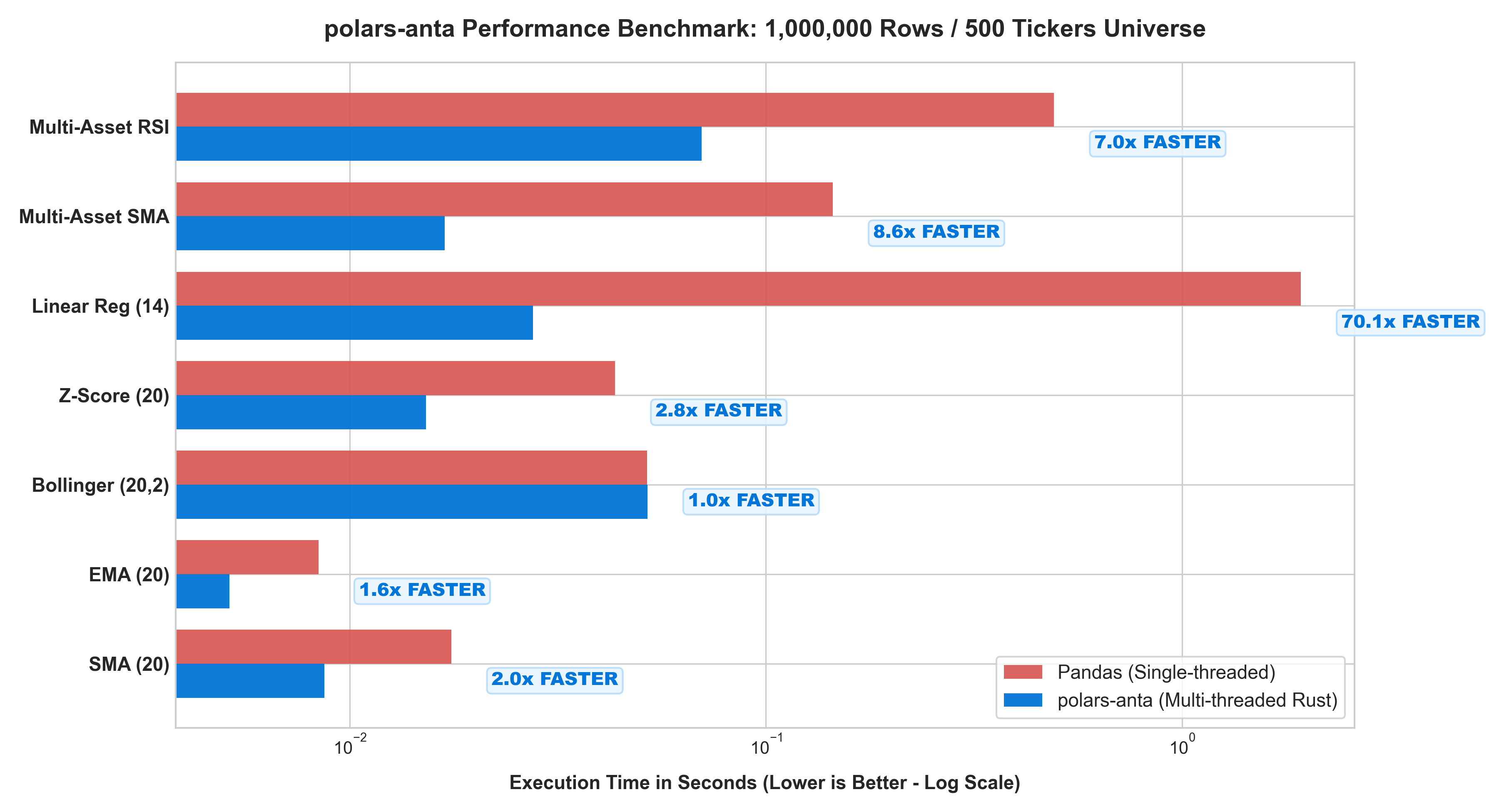
Benchmarks measured across 1,000,000 bars (single-asset random walk) and a 500 tickers × 2,000 bars universe (1,000,000 rows) on Polars' multi-threaded Rust engine vs. single-threaded Pandas:
| Operation / Indicator | Dataset Scale | Pandas Execution | polars-anta Execution |
Measured Speedup |
|---|---|---|---|---|
| Linear Regression Slope (OLS) | 1,000,000 bars | 2.3529 s | 0.0209 s | 112.4x Faster |
| Multi-Asset RSI (14) | 500 tickers × 2k bars | 0.4398 s | 0.0545 s | 8.1x Faster |
| Multi-Asset SMA (20) | 500 tickers × 2k bars | 0.1345 s | 0.0168 s | 8.0x Faster |
| Z-Score Normalization | 1,000,000 bars | 0.0450 s | 0.0267 s | 1.7x Faster |
| Exponential Moving Average | 1,000,000 bars | 0.0100 s | 0.0069 s | 1.5x Faster |
| Simple Moving Average | 1,000,000 bars | 0.0170 s | 0.0153 s | 1.1x Faster |
API Reference & Indicator Catalog
All indicators, alpha primitives, and evaluation functions are exported at the top level (import polars_anta as pa) and registered on .anta and .ta namespaces. Click any module below to expand its complete function signature reference, or visit the Online API Reference.
1. Trend & Overlays — polars_anta.trend · Detailed Docs
| Function Signature | Output Type / Struct Fields | Description |
|---|---|---|
sma(close, period=10) |
Float64 |
Simple Moving Average |
ema(close, period=10) |
Float64 |
Exponential Moving Average |
wma(close, period=10) |
Float64 |
Linearly Weighted Moving Average |
hma(close, period=10) |
Float64 |
Hull Moving Average (low-lag trend filter) |
dema(close, period=10) |
Float64 |
Double Exponential Moving Average |
tema(close, period=10) |
Float64 |
Triple Exponential Moving Average |
zlema(close, period=10) |
Float64 |
Zero-Lag Exponential Moving Average |
t3(close, period=5, vfactor=0.7) |
Float64 |
Tillson T3 Generalized DEMA Smoothing |
alma(close, period=9, offset=0.85, sigma=6.0) |
Float64 |
Arnaud Legoux Gaussian-Filtered Moving Average |
kama(close, period=10, fast_span=2, slow_span=30) |
Float64 |
Kaufman's Efficiency-Adaptive Moving Average |
mcginley_dynamic(close, period=14, k=0.6) |
Float64 |
McGinley Dynamic Volatility-Adjusted Moving Average |
vidya(close, period=9, cmo_period=9) |
Float64 |
Chande's Variable Index Dynamic Average |
heikin_ashi(open, high, low, close) |
Struct(ha_open, ha_high, ha_low, ha_close) |
Vectorized Heikin-Ashi Candlestick Transform (via closed-form ewm_mean(alpha=0.5)) |
supertrend(high, low, close, period=10, multiplier=3.0) |
Struct(supertrend, direction) |
ATR-Based Dynamic Trailing Volatility Stop |
psar(high, low, af_step=0.02, af_max=0.2) |
Float64 |
Welles Wilder's Parabolic Stop and Reverse (SAR) |
ichimoku(high, low, close, tenkan=9, kijun=26, senkou_b=52, displacement=26) |
Struct(tenkan_sen, kijun_sen, senkou_span_a, senkou_span_b, chikou_span) |
Ichimoku Kinko Hyo Equilibrium Cloud |
adx(high, low, close, period=14) |
Struct(adx, plus_di, minus_di) |
Average Directional Movement Index (Wilder's smoothing) |
vortex(high, low, close, period=14) |
Struct(vi_plus, vi_minus) |
Vortex Positive & Negative Trend Movement Indicator |
aroon(high, low, period=25) |
Struct(up, down, oscillator) |
Aroon Trend Age Indicator & Oscillator |
ssl_channel(high, low, close, period=10) |
Struct(ssl_up, ssl_down, hlv) |
Semaphore Signal Level (SSL) Channel |
trend_intensity_index(close, period=30, signal_period=None) |
Float64 or Struct(tii, tii_signal) |
M.H. Pee's Trend Intensity Index (TII) |
chop(high, low, close, period=14) |
Float64 |
E.W. Dreiss Choppiness Index (Trend vs. Consolidation [0, 100]) |
mass_index(high, low, fast_period=9, slow_period=25) |
Float64 |
Donald Dorsey's Range Bulge Reversal Predictor |
center_of_gravity(close, period=10) |
Float64 |
John Ehlers' Center of Gravity (COG) Oscillator |
pivot_points(high, low, close) |
Struct(pivot, r1, r2, r3, s1, s2, s3) |
Classic Floor Trader Pivot Points |
fibonacci_pivots(high, low, close) |
Struct(pivot, r1, r2, r3, s1, s2, s3) |
Fibonacci Retracement/Extension Pivot Points (38.2%, 61.8%, 100%) |
camarilla_pivots(high, low, close) |
Struct(pivot, r1..r4, s1..s4) |
Camarilla Intraday Mean-Reversion & Breakout Pivots |
woodie_pivots(open, high, low, close) |
Struct(pivot, r1, r2, s1, s2) |
Woodie's Close-Weighted Pivot Points |
2. Momentum Oscillators — polars_anta.momentum · Detailed Docs
| Function Signature | Output Type / Struct Fields | Description |
|---|---|---|
rsi(close, period=14) |
Float64 |
Relative Strength Index (Wilder's RMA smoothing) |
macd(close, fast_period=12, slow_period=26, signal_period=9) |
Struct(macd, signal, histogram) |
Moving Average Convergence Divergence |
ppo(close, fast_period=12, slow_period=26, signal_period=9) |
Struct(ppo, signal, histogram) |
Percentage Price Oscillator (scale-invariant MACD) |
stochastic(high, low, close, k_period=14, d_period=3, smooth_k=1) |
Struct(k, d) |
Stochastic Oscillator (%K, %D) |
stoch_rsi(close, rsi_period=14, stoch_period=14, k_smooth=3, d_smooth=3) |
Struct(k, d) |
Chande & Kroll's Stochastic RSI |
squeeze_momentum(high, low, close, bb_period=20, bb_mult=2.0, kc_period=20, kc_mult=1.5) |
Struct(squeeze_on, squeeze_off, no_squeeze, momentum) |
John Carter's TTM Squeeze Volatility Compression & Linear Regression Momentum |
stc(close, fast_period=23, slow_period=50, cycle_period=10, factor=0.5) |
Float64 |
Doug Schaff's Trend Cycle (Double-Stochastic MACD Oscillator [0, 100]) |
tsi(close, long_period=25, short_period=13) |
Float64 |
William Blau's Double-Smoothed True Strength Index |
fisher_transform(high, low, period=10) |
Struct(fisher, signal) |
John Ehlers' Gaussian Fisher Transform |
williams_r(high, low, close, period=14) |
Float64 |
Larry Williams' %R Overbought/Oversold Oscillator [-100, 0] |
cci(high, low, close, period=20, constant=0.015) |
Float64 |
Donald Lambert's Commodity Channel Index (Mean Absolute Deviation) |
roc(close, period=10) |
Float64 |
Percentage Rate of Change |
awesome_oscillator(high, low, fast_period=5, slow_period=34) |
Float64 |
Bill Williams' Midpoint Awesome Oscillator (AO) |
cmo(close, period=14) |
Float64 |
Tushar Chande's Momentum Oscillator [-100, 100] |
coppock(close, wma_period=10, fast_roc=11, slow_roc=14) |
Float64 |
Edwin Coppock's Long-Term Momentum Curve |
ultimate_oscillator(high, low, close, p1=7, p2=14, p3=28) |
Float64 |
Larry Williams' Multi-Timeframe Buying Pressure Oscillator |
rvi(open, high, low, close, period=10) |
Struct(rvi, signal) |
John Ehlers' Symmetrically Weighted Relative Vigor Index |
kst(close, r1=10, r2=15, r3=20, r4=30, ...) |
Struct(kst, signal) |
Martin Pring's "Know Sure Thing" Four-ROC Oscillator |
dpo(close, period=20) |
Float64 |
Detrended Price Oscillator (cycle isolator) |
bop(open, high, low, close) |
Float64 |
Igor Livshin's Balance of Market Power [-1, 1] |
cfo(close, period=14) |
Float64 |
Tushar Chande's OLS Forecast Oscillator (%) |
3. Volatility & Channels — polars_anta.volatility · Detailed Docs
| Function Signature | Output Type / Struct Fields | Description |
|---|---|---|
true_range(high, low, close) |
Float64 |
Welles Wilder's Single-Bar True Range |
atr(high, low, close, period=14) |
Float64 |
Average True Range (Wilder's RMA smoothing) |
natr(high, low, close, period=14) |
Float64 |
Normalized Average True Range (100 * ATR / Close) |
bollinger_bands(close, period=20, num_std=2.0) |
Struct(upper, middle, lower, bandwidth, percent_b) |
John Bollinger's Volatility Envelope, Bandwidth & %B |
bollinger_delta(close, period=20, num_std=2.0) |
Float64 |
Absolute Bollinger Band Spread ($2 \cdot k \cdot \sigma$) |
keltner_channels(high, low, close, ema_period=20, atr_period=10, multiplier=2.0) |
Struct(upper, middle, lower) |
Chester Keltner / Linda Raschke EMA-ATR Volatility Channels |
keltner_width(high, low, close, ema_period=20, atr_period=10, multiplier=2.0) |
Float64 |
Normalized Keltner Channel Width (%) |
donchian_channels(high, low, period=20) |
Struct(upper, middle, lower) |
Richard Donchian's Breakout High/Low Channels |
donchian_width(high, low, period=20) |
Float64 |
Normalized Donchian Channel Width (%) |
chandelier_exit(high, low, close, period=22, multiplier=3.0) |
Struct(long_stop, short_stop) |
Chuck LeBeau's ATR Trailing Chandelier Exit Stops |
starc_bands(high, low, close, period=20, atr_period=15, multiplier=2.0) |
Struct(upper, middle, lower) |
Manning Stoller's Average Range Channels (STARC) |
envelopes(close, period=20, percentage=0.025) |
Struct(upper, middle, lower) |
Percentage Moving Average Envelopes |
stddev(close, period=20) |
Float64 |
Rolling Sample Standard Deviation |
ulcer_index(close, period=14) |
Float64 |
Peter Martin's Downside Drawdown Depth & Duration Risk Index |
historical_volatility(close, period=20, trading_days=252) |
Float64 |
Annualized Close-to-Close Log Return Volatility |
parkinson_volatility(high, low, period=20, trading_days=252) |
Float64 |
Parkinson (1980) Extreme-Value High-Low Range Volatility Estimator |
garman_klass_volatility(open, high, low, close, period=20, trading_days=252) |
Float64 |
Garman & Klass (1980) Minimum-Variance OHLC Volatility Estimator |
chaikin_volatility(high, low, period=10, roc_period=10) |
Float64 |
Marc Chaikin's High-Low Range Expansion Rate of Change |
4. Volume & Money Flow — polars_anta.volume · Detailed Docs
| Function Signature | Output Type / Struct Fields | Description |
|---|---|---|
obv(close, volume) |
Float64 |
Joe Granville's Cumulative On-Balance Volume |
vwap(high, low, close, volume, period=None) |
Float64 |
Volume Weighted Average Price (Cumulative or Rolling Window) |
vwap_bands(high, low, close, volume, period=None, mult1=1.0, mult2=2.0, mult3=3.0) |
Struct(vwap, upper_1..3, lower_1..3) |
Institutional VWAP with Volume-Weighted Standard Deviation Bands |
session_vwap(high, low, close, volume, session_by=None, mult1=1.0, mult2=2.0) |
Struct(vwap, upper_1..2, lower_1..2, zscore) |
Session-Anchored VWAP Resetting per Trading Date/Session with Deviation Z-Score |
vwma(close, volume, period=20) |
Float64 |
Volume Weighted Moving Average |
cmf(high, low, close, volume, period=20) |
Float64 |
Marc Chaikin's Money Flow (CLV-Weighted Volume Ratio) |
adl(high, low, close, volume) |
Float64 |
Chaikin Accumulation / Distribution Line |
mfi(high, low, close, volume, period=14) |
Float64 |
Quong & Soudack's Volume-Weighted RSI (Money Flow Index [0, 100]) |
eom(high, low, volume, period=14, scale=10000.0) |
Float64 |
Richard Arms' Ease of Movement (EMV) |
klinger(high, low, close, volume, fast_period=34, slow_period=55, signal_period=13) |
Struct(klinger, signal) |
Stephen Klinger's Volume Force Oscillator |
nvi(close, volume) |
Float64 |
Norman Fosback's Negative Volume Index (Smart-Money Tracker) |
pvi(close, volume) |
Float64 |
Positive Volume Index (Crowd-Activity Tracker) |
pvt(close, volume) |
Float64 |
Cumulative Return-Weighted Price Volume Trend |
force_index(close, volume, period=13) |
Float64 |
Alexander Elder's EMA-Smoothed Force Index |
vpci(close, volume, short_period=5, long_period=20) |
Float64 |
Buff Dormeier's Volume Price Confirmation Indicator |
vr(close, volume, period=26) |
Float64 |
Up-Volume vs. Down-Volume Ratio (%) |
5. Quantitative Statistics & Regression — polars_anta.stats · Detailed Docs
| Function Signature | Output Type | Description |
|---|---|---|
zscore(close, period=20) |
Float64 |
Rolling Standardized Z-Score Anomaly Metric $(x_t - \mu_t) / \sigma_t$ |
percentile_rank(close, period=20) |
Float64 |
Vectorized Rolling Empirical Percentile Rank $[0.0, 1.0]$ |
skewness(close, period=20) |
Float64 |
Rolling Third Standardized Moment (Return Asymmetry) |
kurtosis(close, period=20) |
Float64 |
Rolling Fourth Standardized Moment (Excess Tail Risk) |
rolling_cov(x, y, period=20) |
Float64 |
Rolling Sample Covariance $\text{Cov}(X, Y)$ |
rolling_corr(x, y, period=20) |
Float64 |
Rolling Pearson Linear Correlation Coefficient $[-1.0, 1.0]$ |
rolling_beta(asset_ret, bench_ret, period=60) |
Float64 |
Rolling CAPM Systematic Market Beta $\text{Cov}(R_a, R_m) / \text{Var}(R_m)$ |
rolling_alpha(asset_ret, bench_ret, rf=0.0, period=60) |
Float64 |
Rolling Jensen's Risk-Adjusted Excess Alpha |
linear_regression_slope(close, period=14) |
Float64 |
Closed-Form Vectorized OLS Linear Regression Slope ($\beta_1$) |
linear_regression_intercept(close, period=14) |
Float64 |
Closed-Form Vectorized OLS Linear Regression Intercept ($\beta_0$) |
linear_regression_angle(close, period=14) |
Float64 |
Rolling OLS Regression Trend Angle in Degrees $\arctan(\beta_1) \cdot \frac{180}{\pi}$ |
linear_regression_forecast(close, period=14) |
Float64 |
Rolling OLS End-of-Window Fitted Value $\hat{y}_t = \beta_0 + \beta_1 (n - 1)$ |
frac_diff(close, d=0.4, window=20) |
Float64 |
Fixed-Window Fractional Differentiation (FFD — López de Prado, 2018) $(1 - B)^d$ |
6. Alpha Factor & Microstructure Primitives — polars_anta.alpha · Detailed Docs
| Function Signature | Domain | Description |
|---|---|---|
cs_rank(expr, over=None, method="average", percentile=True) |
Cross-Sectional | Cross-sectional percentile rank $[0.0, 1.0]$ |
cs_zscore(expr, over=None, clip_bound=None) |
Cross-Sectional | Cross-sectional zero-mean unit-variance standardization with optional $z$-clipping |
cs_winsorize(expr, over=None, method="quantile", lower=0.01, upper=0.99, threshold=3.0) |
Cross-Sectional | Cross-sectional outlier clipping via "quantile", "zscore", or robust "mad" |
neutralize(expr, by, over=None, standardize=False) |
Cross-Sectional | Sector/industry/group demeaning & standardization |
orthogonalize(expr, factors, over=None, standardize=True, ridge=0.0) |
Cross-Sectional | Multi-factor OLS Gram-Schmidt residualization & standardization |
ts_scale(expr, a=1.0, over=None) |
Cross-Sectional | L1 book-size normalization ($\sum \vert w_i\vert = a$) |
amihud_illiquidity(close, volume, period=20, scale=1e6) |
Microstructure | Amihud (2002) Illiquidity Ratio $\frac{1}{N}\sum \frac{\vert r_t\vert }{\text{DollarVolume}_t} \times \text{scale}$ |
roll_spread(close, period=20) |
Microstructure | Roll (1984) Serial Price-Change Covariance Effective Bid-Ask Spread $2\sqrt{\max(0, -\text{Cov}(\Delta P_t, \Delta P_{t-1}))}$ |
corwin_schultz_spread(high, low, period=20) |
Microstructure | Corwin & Schultz (2012) Two-Bar High-Low Range Effective Bid-Ask Spread Estimator |
kyle_lambda(close, volume, period=20, scale=1e6) |
Microstructure | Kyle (1985) Price-Impact Coefficient $\lambda$ via Rolling OLS on Signed Dollar Volume |
vpin(close, volume, period=20) |
Microstructure | Bulk Volume Classification (BVC) Volume-Synchronized Probability of Informed Trading $[0, 1]$ |
ofi(bid_price, bid_size, ask_price, ask_size, period=1) |
Microstructure | Cont, Kukanov & Stoikov (2014) Level-1 Order Flow Imbalance |
futures_basis(futures_close, spot_close, days_to_expiry=None, period=20) |
Index Futures | Futures-Spot Spread, Proportional Basis, Annualized Carry & Basis Z-Score (Struct) |
oi_regime(close, open_interest, period=1) |
Index Futures | 4-State Open Interest & Price Action Regime Classifier (Struct: Long/Short Buildup & Covering/Liquidation) |
twap(high, low, close, period=20) |
Microstructure | Rolling Time-Weighted Average Price |
relative_spread(high, low, close) |
Microstructure | Intraday High-Low Relative Range Proxy $(H_t - L_t) / C_t$ |
hl_ratio(high, low) |
Microstructure | Log Intraday Volatility Expansion $\ln(H_t / L_t)$ |
co_ratio(close, open) |
Microstructure | Log Intraday Sentiment Drift $\ln(C_t / O_t)$ |
returns_divergence(close, volume, period=14) |
Microstructure | Rolling Price Return vs. Volume Change Divergence |
volume_weighted_momentum(close, volume, period=10) |
Microstructure | Price Rate of Change Amplified by Relative Volume Ratio |
ts_rank(close, period=10) |
Time-Series | Vectorized rolling percentile rank $[0.0, 1.0]$ |
ts_argmax(close, period=10) |
Time-Series | Vectorized bars elapsed since rolling window peak |
ts_argmin(close, period=10) |
Time-Series | Vectorized bars elapsed since rolling window trough |
decay_linear(close, period=10) |
Time-Series | Linearly decaying weighted moving average |
ts_delta(expr, period=1) |
Time-Series | Difference operator $x_t - x_{t-d}$ |
ts_delay(expr, period=1) |
Time-Series | Lag operator $x_{t-d}$ |
signed_power(expr, exponent=2.0) |
Time-Series | Sign-preserving power $\text{sign}(x) \cdot \vert x\vert ^a$ |
ts_min(expr, period=10) |
Time-Series | Rolling window minimum |
ts_max(expr, period=10) |
Time-Series | Rolling window maximum |
ts_sum(expr, period=10) |
Time-Series | Rolling window sum |
ts_std(expr, period=10) |
Time-Series | Rolling sample standard deviation |
ts_product(expr, period=10) |
Time-Series | Vectorized rolling window product |
ts_correlation(x, y, period=10) |
Time-Series | Rolling Pearson correlation |
ts_covariance(x, y, period=10) |
Time-Series | Rolling sample covariance |
ts_zscore(close, period=20) |
Time-Series | Time-series rolling standardization $(x_t - \mu_t) / \sigma_t$ |
hurst_exponent(close, period=50) |
Regime / Complexity | Vectorized Rolling R/S Hurst Exponent $H \in [0, 1]$ (mean-reversion vs. trend persistence) |
fractal_dimension(high, low, period=20) |
Regime / Complexity | John Ehlers' Fractal Dimension Index $D \in [1, 2]$ (market noise vs. trend efficiency) |
entropy(close, period=20, bins=5) |
Regime / Complexity | Rolling Normalized Shannon Information Entropy $[0, 1]$ |
alpha_001 – alpha_030 |
Formulaic Alpha | Canonical formulaic alphas (#1 through #30, Kakushadze 2016) |
alpha_041(high, low, close, volume) |
Formulaic Alpha | Geometric High-Low Midpoint vs. VWAP |
alpha_054(open, high, low, close) |
Formulaic Alpha | Intraday Candlestick Power Ratio |
alpha_101(open, high, low, close) |
Formulaic Alpha | Normalized Intraday Body-to-Range Momentum |
7. Factor Evaluation, Performance Metrics & Vectorized Backtesting — polars_anta.evaluation, backtest · Detailed Docs
| Function Signature | Domain | Description |
|---|---|---|
forward_returns(df, close_col="close", periods=(1, 5, 10), group_by=None) |
Factor Evaluation | Multi-horizon forward returns $(P_{t+k} / P_t) - 1$ for factor testing |
information_coefficient(df, factor_col, return_col, group_by=None, method="spearman") |
Factor Evaluation | Cross-sectional Rank IC ("spearman") or Normal IC ("pearson") series |
ic_summary(df, factor_col, return_col, group_by=None, method="spearman", nw_lags=None) |
Factor Evaluation | Summary dictionary (ic_mean, ic_std, icir, t_stat, nw_t_stat, hit_rate, n_periods) |
ic_decay(df, factor_col, close_col="close", horizons=(1, 2, 3, 5, 10, 20), ...) |
Factor Evaluation | Multi-horizon IC decay schedule with Newey-West HAC $t$-stat and exponential Alpha Half-Life |
quantile_analysis(df, factor_col, return_col, quantiles=5, group_by=None) |
Factor Evaluation | Quantile bucket returns, Sharpe, win rate, and cumulative performance ($Q_1 \dots Q_N$) |
factor_turnover(df, factor_col, asset_col="ticker", time_col="timestamp", lag=1) |
Factor Evaluation | Rank autocorrelation and L1 signal turnover across periods |
triple_barrier_labels(close, volatility=None, horizon=10, pt_mult=2.0, sl_mult=2.0, ...) |
AFML Labeling | Dynamic Triple-Barrier & Meta-Labeling (Struct(label, touch_bars, realized_return, meta_label)) |
trend_scanning_labels(close, min_window=5, max_window=20, step=1) |
AFML Labeling | Multi-Horizon OLS Trend-Scanning Labels (Struct(label, t_value, optimal_window, ret)) |
drawdown_series(returns_or_equity, is_returns=True) |
Performance Metric | Underwater percentage drawdown curve $\le 0.0$ |
max_drawdown(returns_or_equity, is_returns=True) |
Performance Metric | Scalar Maximum Drawdown (MDD) |
sharpe_ratio(returns, risk_free_rate=0.0, annualization=252.0) |
Performance Metric | Annualized Sharpe Ratio scalar expression |
sortino_ratio(returns, risk_free_rate=0.0, annualization=252.0) |
Performance Metric | Annualized Sortino Ratio using downside deviation |
calmar_ratio(returns, annualization=252.0) |
Performance Metric | Annualized Return divided by $\vert MDD\vert $ |
profit_factor(returns) |
Performance Metric | Gross Profit divided by $\vert Gross Loss\vert $ |
win_rate(returns, include_zeros=False) |
Performance Metric | Proportion of active periods with positive returns |
probabilistic_sharpe_ratio(returns, benchmark_sr=0.0, risk_free_rate=0.0, annualization=252.0) |
Performance Metric | Skewness- & Kurtosis-adjusted Probabilistic Sharpe Ratio (PSR $\in [0, 1]$) |
deflated_sharpe_ratio(returns, n_trials=10, trials_sr_std=0.5, ...) |
Performance Metric | Multiple-Testing Deflated Sharpe Ratio (DSR $\in [0, 1]$, Bailey & López de Prado 2014) |
crosses_above(a, b, over=None) / crosses_below(a, b, over=None) |
Backtesting | Boolean crossover/crossunder detection against another series or scalar threshold |
signals_to_positions(entries, exits, ...) |
Backtesting | Loop-free .forward_fill() state machine converting entry/exit triggers to positions |
vectorized_backtest(df, signal="signal", ...) / df.anta.backtest(...) |
Backtesting | Vectorized backtester with execution_price (open/twap/vwap), flat_mask, vol_target, no_trade_buffer, fees & slippage |
BacktestResult / extract_trades(bt_df) |
Backtesting | Result container (.data, .summary, .report(), .trades()) & Round-Trip Trade Ledger with MAE/MFE |
parameter_sweep(df, signals, ...) / compare_strategies(strategies) |
Backtesting | Multi-parameter grid evaluation with automatic Deflated Sharpe Ratio (dsr) & strategy comparison |
8. Data Engineering, Information Bars & Futures Roll — polars_anta.resample · Detailed Docs
| Function Signature | Domain | Description |
|---|---|---|
validate_ohlcv(df, ...) / df.anta.validate_ohlcv(...) |
Data Integrity | Structural validation of OHLCV invariants ($H_t \ge \max(O_t, C_t, L_t)$, $L_t \le \min(O_t, C_t, H_t)$, $V_t \ge 0$, chronological monotonicity) |
resample_ohlcv(df, every, ...) / df.anta.resample(every, ...) |
Time Bar Aggregation | Multi-timeframe calendar aggregation ("5m", "15m", "1h", "1d") via group_by_dynamic |
resample_volume_bars(df, volume_threshold, ...) |
Information Bars | Cumulative Volume Bar sampling ($\sum V_i \ge \Theta_V$) restoring return Gaussianity |
resample_dollar_bars(df, dollar_threshold, ...) |
Information Bars | Cumulative Dollar/Notional Bar sampling ($\sum P_i V_i \ge \Theta_D$) invariant to price inflation |
resample_imbalance_bars(df, expected_imbalance, ...) |
Information Bars | López de Prado (2018) Tick/Volume Imbalance Bars ($\left\vert \sum b_i v_i\right\vert \ge \Theta_{\text{TIB/VIB}}$) |
stitch_futures_roll(df, method="backward", ...) |
Continuous Futures | Non-leaky continuous futures stitching ("backward", "ratio", "panama") across contract expiries |
Quantitative Theory, Mathematical Foundations & Rust Vectorization Architecture
For complete derivations, step-by-step proofs, and institutional research workflows, see Architecture & Mathematical Proofs and Quantitative Theory & Institutional Workflows.
1. Closed-Form Algebraic Reductions ($O(N)$ Rust Native Kernels)
-
112.4x Faster Rolling OLS Linear Regression (
linear_regression_slope): Instead of solving $\left(X^\top X\right)^{-1} X^\top Y_t$ inside a Python loop over $N$ bars,polars-antaexploits the exact linear relationship between the Linearly Weighted Moving Average ($\text{WMA}_n$, weights $w_i \propto i+1$) and Simple Moving Average ($\text{SMA}_n$):$$\beta_{1,t} = \frac{6}{n + 1}\left(\text{WMA}_n(y)_t - \text{SMA}_n(y)t\right), \qquad \beta{0,t} = \text{SMA}_n(y)t - \beta{1,t}\frac{n - 1}{2}$$
Both $\text{WMA}_n$ and $\text{SMA}_n$ execute natively inside Polars' multi-threaded Rust engine with $O(1)$ amortized cost per bar.
-
Wilder's RMA & Heikin-Ashi via Exact
ewm_meanMapping: Wilder's recursive smoothing ($RMA_t = \frac{1}{n}x_t + \frac{n-1}{n}RMA_{t-1}$ inrsi,atr,adx) and Heikin-Ashi open prices ($HA_Open_t = \frac{1}{2}HA_Open_{t-1} + \frac{1}{2}HA_Close_{t-1}$) are mapped directly topl.Expr.ewm_mean(alpha=1/n, adjust=False)andewm_mean(alpha=0.5, adjust=False)—eliminating sequential Python loops completely. -
Fixed-Window Fractional Differentiation (
frac_diff, López de Prado 2018): Expands the backshift operator $(1 - B)^d = \sum_{k=0}^{\infty} \omega_k B^k$ via recursive binomial weights $\omega_0 = 1, ; \omega_k = -\omega_{k-1} \frac{d - k + 1}{k}$ over a fixed window $W$, achieving statistical stationarity ($d \approx 0.3\text{–}0.5$) while preserving long-memory trend/cointegration information lost by first-differencing ($d=1$).
2. Cross-Sectional Factor Orthogonalization & Statistical Inference
-
Modified Gram-Schmidt Multi-Factor Projection (
orthogonalize): Applies the Frisch-Waugh-Lovell theorem per timestamp cross-section (over="date") to strip linear exposures to $K$ arbitrary risk factors $F = [f_1, \dots, f_K]$ (e.g., Market Beta, Log Size, Volatility, Liquidity) with optional Ridge regularization $\lambda \ge 0$:$$u_k = \tilde{f}k - \sum{j=1}^{k-1} \frac{\langle \tilde{f}k, u_j \rangle}{|u_j|2^2 + \lambda} u_j, \qquad \epsilon\alpha = \tilde{\alpha} - \sum{k=1}^{K} \frac{\langle \tilde{\alpha}, u_k \rangle}{|u_k|_2^2 + \lambda} u_k$$
-
Newey-West HAC $t$-Statistics & Exponential Alpha Half-Life (
ic_summary,ic_decay): Multi-period forward returns ($h > 1$) induce $MA(h-1)$ serial correlation in Information Coefficient series.polars-antaapplies the Newey & West (1987) Bartlett kernel variance estimator $\hat{\Omega}{NW} = \hat{\gamma}0 + 2 \sum{j=1}^{L} \left(1 - \frac{j}{L+1}\right) \hat{\gamma}j$ so $t{NW} = \frac{\overline{IC}}{\sqrt{\hat{\Omega}{NW} / T}}$ remains unbiased, and fits $\ln |IC(h)| = a - \lambda h$ to estimate the exact signal Half-Life $t_{1/2} = \frac{\ln 2}{\lambda}$. -
Probabilistic & Deflated Sharpe Ratios (
probabilistic_sharpe_ratio,deflated_sharpe_ratio): Adjusts Sharpe Ratio inference for non-normal skewness ($\hat{\gamma}_3$), fat tails ($\hat{\gamma}_4$), and selection bias across $K$ tested parameter configurations (Bailey & López de Prado, 2014):$$\text{PSR}(SR^) = \Phi!\left(\frac{(\widehat{SR} - SR^)\sqrt{T - 1}}{\sqrt{1 - \hat{\gamma}_3 \widehat{SR} + \frac{\hat{\gamma}4 - 1}{4}\widehat{SR}^2}}\right), \qquad SR^*{DSR} = \sqrt{V[{\widehat{SR}_k}]}\left((1 - \gamma)\Phi^{-1}!\left(1 - \frac{1}{K}\right) + \gamma \Phi^{-1}!\left(1 - \frac{1}{K e}\right)\right)$$
3. Zero-Copy Stride Windows & Loop-Free State Machines
- Zero-Copy 2D Stride Views: Path-dependent rolling operators (
triple_barrier_labels,trend_scanning_labels,hurst_exponent,entropy,ts_rank,ts_argmax) construct virtual 2D rolling views(N - P + 1, P)vianumpy.lib.stride_tricks.sliding_window_viewwith $O(1)$ pointer/stride metadata overhead and zero memory duplication. - State-Machine Backtesting & Excursion Analytics (
vectorized_backtest,extract_trades): Entry/exit signals compile into positions via.forward_fill(), apply ex-ante volatility targeting ($w_t^{\text{vol}} = \text{clip}(\sigma_{\text{target}} / \hat{\sigma}{t-1}, 0, L{\max})$), enforce intraday flatten masks (flat_mask), execute at next-bar Open/TWAP/VWAP prices (execution_price), and group active position runs via.rle_id()to compute exact per-trade Maximum Adverse Excursion (MAE) and Maximum Favorable Excursion (MFE).
Design philosophy
polars-anta aims to balance mathematical clarity, cross-sectional expressiveness, and execution speed:
- Keep quantitative formulas inspectable — write indicators using closed-form algebraic identities and native Polars expressions (
pl.Expr) rather than hiding logic behind compiled C extensions. - Eliminate Python loops — express recursive smoothing (Wilder's RMA, Heikin-Ashi) via exact
ewm_meanrecurrences and path-dependent rolling operators via zero-copysliding_window_viewkernels. - Treat single-asset and multi-asset panels uniformly — every expression composes naturally with
.over("ticker")for time-series operations and.over("date")for cross-sectional ranking and neutralization. - Prevent look-ahead bias by default — backtesting utilities shift signals by
signal_lag=1bar out of the box and account for proportional transaction fees and slippage. - Provide reproducible examples and parity tests — verify mathematical accuracy through comprehensive unit test suites and self-contained notebooks.
Contributing
Contributions from quantitative researchers, developers, and finance students are welcome! You can help by implementing new indicators, expanding formulaic alphas, improving documentation, or adding tutorial notebooks.
- Browse our open Good First Issues & Help Wanted tasks to find a self-contained issue with full mathematical specifications.
- Read CONTRIBUTING.md for development setup, testing (
pytest -v), and linting (ruff check .) guidelines.
Project status and support
polars-anta is an actively developed open-source project. If you find a bug, need an indicator, or want to suggest a quantitative workflow example, please open an issue or join GitHub Discussions.
Disclaimer: polars-anta is provided for educational and research purposes without warranty of any kind. Quantitative models and backtest results should be independently verified before being used for live trading, investment, or risk-management decisions.
Author
polars-anta was created and is maintained by Phan Bui Huu An (@huuan26 • phanbuihuuan261103@gmail.com).
License
polars-anta is licensed under the Apache License 2.0. See the LICENSE file for details.
Explore the indicators • Run the Colab notebooks • Contribute to open quantitative finance
1 maintainer

Metadata
1 maintainer
Release files for polars-anta 0.3.1
For a detailed explanation of source distributions (sdists) and built distributions (wheels), please see the package formats documentation.
Source distribution (sdist)
| File | Size | Uploaded | Provenance | Actions |
|---|---|---|---|---|
| polars_anta-0.3.1.tar.gz | 1.1 MB | With provenance | Details for polars_anta-0.3.1.tar.gz |
Built distribution (wheel)
| File | Interpreter | ABI | Platform | Actions Reset |
|---|---|---|---|---|
| polars_anta-0.3.1-py3-none-any.whl | Python 3 | none | any | Details for polars_anta-0.3.1-py3-none-any.whl |
Total release size: 1.2 MB
Release files / polars_anta-0.3.1.tar.gz
| Download URL | polars_anta-0.3.1.tar.gz |
|---|---|
| Size | 1.1 MB |
| Tags | Source |
|
SHA-256 checksum How to use checksums |
952c14982f2aeb6e76c79080c0260b76a30ab41946d087c343c981c850dc9959
|
|
BLAKE2b-256 checksum How to use checksums |
f7f35892027323cd81f400f97f710ff756c69af4061e59e4fde699abcbd856db
|
| Upload date | |
|
Uploaded using Trusted Publishing? What is trusted publishing? |
Yes |
| Uploaded via |
twine/7.0.0 CPython/3.13.16
|
Provenance
Provenance describes where a file came from. On PyPI, provenance is shared via attestations, which provide a verifiable record of the build or publishing details. View details, limitations and caveats.


PyPI Publish Attestation
PyPI verified that this artifact, at this checksum, originated from the publisher listed below.
Signed by GitHub Actions, verified by PyPI on Nov 1, 2026.
Transparency logRelease files / polars_anta-0.3.1-py3-none-any.whl
| Download URL | polars_anta-0.3.1-py3-none-any.whl |
|---|---|
| Size | 104.5 kB |
| Tags | Python 3 |
|
SHA-256 checksum How to use checksums |
0c10480c4326b6adec9683d36b3d27ca9e1596dd42795f29670162fc4018bdbb
|
|
BLAKE2b-256 checksum How to use checksums |
0088f30df9608b3ff243080b5c9fa45d9b5da66f26dcad0e1fd63b209fb31e73
|
| Upload date | |
|
Uploaded using Trusted Publishing? What is trusted publishing? |
Yes |
| Uploaded via |
twine/7.0.0 CPython/3.13.16
|
Provenance
Provenance describes where a file came from. On PyPI, provenance is shared via attestations, which provide a verifiable record of the build or publishing details. View details, limitations and caveats.
PyPI Publish Attestation
PyPI verified that this artifact, at this checksum, originated from the publisher listed below.
Signed by GitHub Actions, verified by PyPI on Nov 1, 2026.
Transparency logSecurity for polars-anta 0.3.1
Provenance
Provenance describes where a file came from. On PyPI, provenance is shared via attestations, which provide a verifiable record of the build or publishing details. View details, limitations and caveats.
Full provenance
Both files in this release have been uploaded with provenance metadata.
Attestation for polars_anta-0.3.1.tar.gz
PyPI Publish Attestation
PyPI verified that this artifact, at this checksum, originated from the publisher listed below.
Signed by GitHub Actions, verified by PyPI on Nov 1, 2026.
Transparency logA note on package security
PyPI is a repository for distributing packages, not a service for auditing them. While third-party security researchers and our staff do their best to detect and remove malicious packages, PyPI cannot guarantee the quality, security or suitability of any given package.
To learn more about protecting yourself from malicious actors, visit our package security documentation.














