A package for asset allocation

Project description
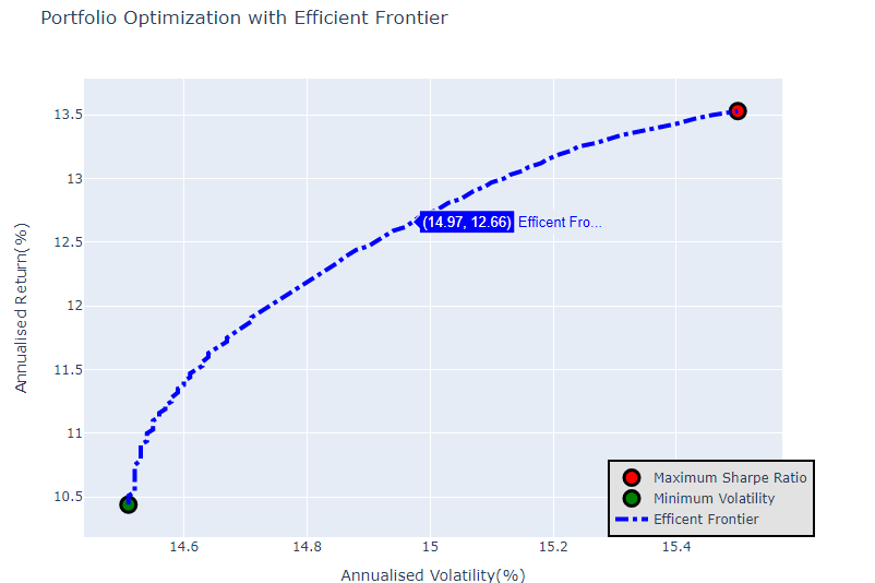
Efficient-Frontier
We implement an Efficient Frontier that plots the optimal expected portfolio return against a certain level of risk measured by portfolio variance. This is achieved by constraint optimisation using predefined portfolio constraints and iterating across expected levels of return from the Lowest-Variance portfolio to the maximum possible return of the portfolio with the maximum Sharpe Ratio. We define various constraints to calculate the weightings for the minVar portfolio(Minimum Variance), the MaxSR(Maximum Sharpe Ratio Portfolio) and the optimisation required to calculate variances after the optimal return weightings for all the target returns that lie between. This requires us to define portfolio performance functions which will be the focus of our code in the beginning.
First we need to import all the following libraries.
python -m pip install yfinance
python -m pip install plotly
python -m pip install scipy
python -m pip install pandas
python -m pip install datetime
pip install -i https://test.pypi.org/simple/ portfiel
Firstly we'd need to set up the covariance matrix and the expected returns of the multiple stocks to be added to multi-stock porttfolio. We extract data using the pandas datareader(Yahoo) and set up the requisites in the following section.
#Importing Data from YFin
def getData(stocks, start, end):
  stockData = pdr.get_data_yahoo(stocks, start = start, end = end)
  stockData = stockData['Close']

  returns = stockData.pct_change()
  meanReturns = returns.mean()
  covMatrix = returns.cov()
  return meanReturns, covMatrix
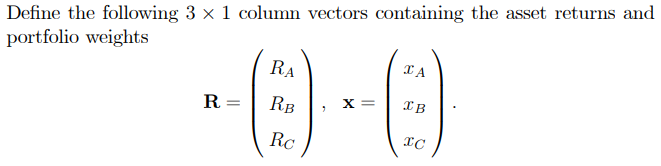
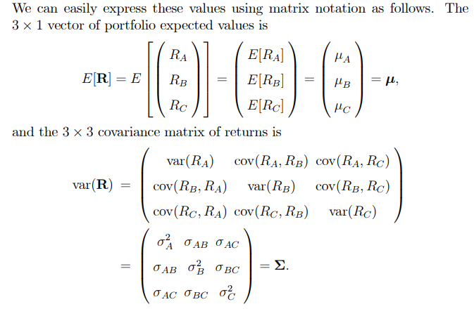
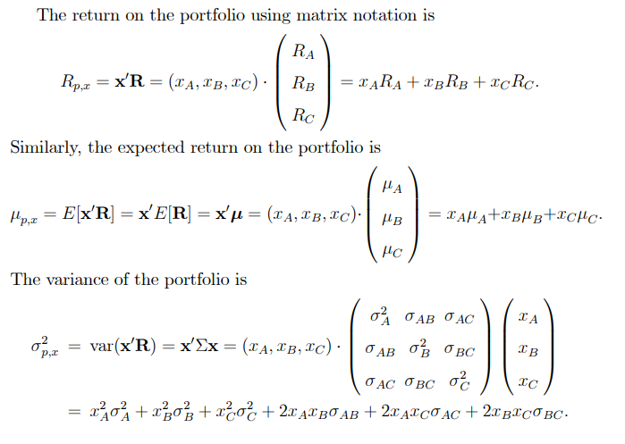
For a Generalised Multi-Stock Portfolio LinAlg implementation using a 3-stock portfolio as an example, we have the following theoretical computations:
#Defining Portfolio Performance
def portfolioPerformance(weights, meanReturns, covMatrix):
  returns = np.sum(meanReturns * weights) * 252   #No. of Trading Day
  std = np.sqrt(np.dot(weights.T, np.dot(covMatrix, weights))) * np.sqrt(252)    #Volatility is Sigma*Sqrt(T)
  #Converting equation above to matrix form. Variance is add-able and we use 252 as it is the number of trading days.
  return returns, std
Now we use SLSQP Minimisation for most of our purposes as it is easy to use and is offered by Scipy. The first of the optimisations involve, building the portfolio with Maximum Sharpe Ratio, however as we have a minimisation algorithm, we need to define a negativeSR function that would be minimised in order to find the weightings for the MaxSR portfolio based on the following constraints.
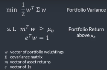
The sc.minimize function first takes the function to be optimised as the first argument, the optimisation would take place over the first argument of the function to be optimised. Essentially, if negativeSR is the argument to sc.minimize, the minimisation of negativeSR would take place by varying the first argument of negativeSR, i.e, weights. The second argument for sc.minimise is the initialisation for the weights parameter. In this case we make a vector as long as the number of assets with equal weights(1/Number of Assets). Bounds are defined as the set of values that can be taken by the weights parameter for each stock, and constraints define the ones delineated in the image above.
def negativeSR(weights, meanReturns, covMatrix, riskFreeRate = 0):
  pReturns, pStd = portfolioPerformance(weights, meanReturns, covMatrix)
  return -(pReturns - riskFreeRate)/pStd
  #Returning NSharpe Ratio as -(Excess Return over Market/Risk Taken)

def maxSR(meanReturns, covMatrix, riskFreeRate = 0, constraintSet = (0,1)):
  # Minimise the NegativeSR by altering the weights of the portfolio.
  numAssets = len(meanReturns)
  args = (meanReturns, covMatrix, riskFreeRate)
  constraints = ({'type':'eq', 'fun': lambda x : np.sum(x) - 1})
  bound = constraintSet
  bounds = list(bound for asset in range(numAssets))
  result = sc.minimize(negativeSR, numAssets * [1./ numAssets], args = args, method = 'SLSQP', bounds = bounds, constraints = constraints)
  return result
Similarly we define a minVar function:
def minimizeVariance(meanReturns, covMatrix, riskFreeRate = 0, constraintSet = (0,1)):
  #Minimise the portfolio variance by altering the weights/allocation of assets in the portfolio
  numAssets = len(meanReturns)
  args = (meanReturns, covMatrix)
  constraints = ({'type':'eq', 'fun': lambda x : np.sum(x) - 1})
  bound = constraintSet
  bounds = list(bound for asset in range(numAssets))
  result = sc.minimize(portfolioVariance, numAssets * [1./ numAssets], args = args, method = 'SLSQP', bounds = bounds, constraints = constraints)

  return result
Now that we have the range of target returns, all we need to do is iterate and minimize portfolio variance for all target return values that lie between the lowest variance and optimal variance. We have to prepare a generalised optimisation function that though similar to previous optimisers, additionally takes as a constraint, the target return.
def efficientOpt(meanReturns, covMatrix, returnTarget, constraintSet = (0,1)):
  'For each returnTarget, we want to optimise the portfolio for minimum variance.'
  numAssets = len(meanReturns)
  args = (meanReturns, covMatrix)
  constraints = ({'type':'eq', 'fun':lambda x: portfolioReturn(x, meanReturns, covMatrix)- returnTarget},{'type':'eq', 'fun': lambda x : np.sum(x) - 1})  #Can be an inequality(>=)
  bound = constraintSet
  bounds = tuple(bound for asset in range(numAssets))
  effOpt = sc.minimize(portfolioVariance, numAssets * [1./numAssets], args = args, constraints = constraints, method = 'SLSQP', bounds = bounds)

  return effOpt
Now finally we have a main function to call all of these previously defined functions and returns the Expected Return, Variance and the portfolio weights for each iteration. We will use this to plot the frontier in the subsequent step.
def calculatedResults(meanReturns, covMatrix, riskFreeRate = 0, constraintSet = (0,1)):
  '''Function to read Mean, CovMatrix and other Financial Information
  Output Maximum Sharpe Ratio, Min Volatility and Efficient Frontier'''

  #For Maximum Sharpe Ratio
  maxSR_Portfolio = maxSR(meanReturns,covMatrix)
  maxSR_Returns, maxSR_std = portfolioPerformance(maxSR_Portfolio['x'], meanReturns, covMatrix)
  maxSR_allocation = pd.DataFrame(maxSR_Portfolio['x'], index = meanReturns.index, columns = ['Allocation'])
  maxSR_allocation.Allocation = [round(i*100,0) for i in maxSR_allocation.Allocation]

  #For Min Volatitlity Portfolio
  minVol_Portfolio = minimizeVariance(meanReturns,covMatrix)
  minVol_Returns, minVol_std = portfolioPerformance(minVol_Portfolio['x'], meanReturns, covMatrix)
  minVol_allocation = pd.DataFrame(minVol_Portfolio['x'], index = meanReturns.index, columns = ['Allocation'])
  minVol_allocation.Allocation = [round(i*100,0) for i in minVol_allocation.Allocation]


  #Efficient Frontier
  efficientList = []
  targetReturns = np.linspace(minVol_Returns, maxSR_Returns, 100)
  for target in targetReturns:
    efficientList.append(efficientOpt(meanReturns, covMatrix, target)['fun'])

  maxSR_Returns, maxSR_std = round(maxSR_Returns * 100,2), round(maxSR_std*100,2)
  minVol_Returns, minVol_std = round(minVol_Returns * 100,2), round(minVol_std*100,2)

  return maxSR_Returns, maxSR_std, maxSR_allocation, minVol_Returns, minVol_std, minVol_allocation, efficientList, targetReturns
Finally we use plotly to plot the efficient frontier.
def EF_graph(meanReturns, covMatrix, riskFreeRate = 0, constraintSet = (0,1)):
  'Return a graph plotting the Min. Volatility, MaxSR and EfficientFrontier'
  maxSR_Returns, maxSR_std, maxSR_allocation, minVol_Returns, minVol_std, minVol_allocation, efficientList, targetReturns = calculatedResults(meanReturns, covMatrix)

  #Max SR
  MaxSharpeRatio = go.Scatter(
      name = 'Maximum Sharpe Ratio',
      mode = 'markers',
      x = [maxSR_std],
      y = [maxSR_Returns],
      marker = dict(color = 'red', size = 14, line = dict(width = 3, color = 'black'))
  )

  #Min Vol.
  MinVol = go.Scatter(
      name = 'Minimum Volatility',
      mode = 'markers',
      x = [minVol_std],
      y = [minVol_Returns],
      marker = dict(color = 'green', size = 14, line = dict(width = 3, color = 'black'))
  )

  #Efficient Frontier
  EF_curve = go.Scatter(
      name = 'Efficent Frontier',
      mode = 'lines',
      x = [round(ef_std*100, 2) for ef_std in efficientList],
      y = [round(target*100, 2) for target in targetReturns],
      line = dict(color = 'blue', width = 4, dash = 'dashdot')
  )

  data = [MaxSharpeRatio, MinVol, EF_curve]

  layout = go.Layout(
      title = 'Portfolio Optimization with Efficient Frontier',
      yaxis = dict(title = 'Annualised Return(%)'),
      xaxis = dict(title = 'Annualised Volatility(%)'),
      width = 800,
      height = 600,
      showlegend = True,
      legend = dict(
          x = 0.75, y = 0, traceorder = 'normal',
          bgcolor = '#E2E2E2',
          bordercolor = 'black',
          borderwidth = 2),
          )

  fig = go.Figure(data = data,layout = layout)
  return fig.show()

EF_graph(meanReturns, covMatrix)
Release history Release notifications | RSS feed

Download files
Download the file for your platform. If you're not sure which to choose, learn more about installing packages.
Source Distribution
Built Distribution
Filter files by name, interpreter, ABI, and platform.
If you're not sure about the file name format, learn more about wheel file names.
Copy a direct link to the current filters
File details
Details for the file portfiel-0.1.4.tar.gz.
File metadata
- Download URL: portfiel-0.1.4.tar.gz
- Upload date:
- Size: 8.4 kB
- Tags: Source
- Uploaded using Trusted Publishing? No
- Uploaded via: twine/4.0.1 CPython/3.10.5
File hashes
| Algorithm | Hash digest | |
|---|---|---|
| SHA256 |
f6d82de21a9bdecb231a0b59008384a7cbf22dac96c711277b20595ac6df47f0
|
|
| MD5 |
9f5ee7ec5a893e030a1265786a4bd642
|
|
| BLAKE2b-256 |
3765eefcc69e7f834b1c636000da1b842dbeba111db7783297e9540d5fcf1d7c
|
File details
Details for the file portfiel-0.1.4-py3-none-any.whl.
File metadata
- Download URL: portfiel-0.1.4-py3-none-any.whl
- Upload date:
- Size: 7.8 kB
- Tags: Python 3
- Uploaded using Trusted Publishing? No
- Uploaded via: twine/4.0.1 CPython/3.10.5
File hashes
| Algorithm | Hash digest | |
|---|---|---|
| SHA256 |
5fa91fe6715c1ca74efe5de8823dc8ce64f2f8325b263e4044c088db404d3df8
|
|
| MD5 |
0c1c92c65944b88f9273f141317d8be3
|
|
| BLAKE2b-256 |
ac55319d38f258051775617aca4bb8073f599a3e26a900b6c25ae17a90e0bfd9
|


