
ppgrid - Pull-Push Scattered-Data Interpolation
Fast, continent-scale raster interpolation for scattered point data. Turns tens of millions of geolocated points into a pair of GeoTIFFs in minutes on a single machine. No GPU needed.
What it does
You have N points (N ~ 10^7) with (longitude, latitude, value). You want a raster of M cells where every cell within a defensible distance of real data carries an interpolated value, and everything else is nodata.
Standard IDW in QGIS/ArcGIS is O(N×M) (~14 hours for 16M points. This tool uses pull-push mipmap interpolation to reduce cost to O(M), independent of N.
How it works
Pull-Push (mipmap) Interpolation
From Gortler et al. 1996 (Lumigraph) and Kraus 2009.
Once points are snapped to a grid, IDW is exactly a normalised convolution:
z = (S ⊛ K) / (C ⊛ K) K(r) = r^-p
Pull-push evaluates this across a mipmap pyramid so cost is O(M), independent of N.
Steps:
- Points are binned into
S(sum of transformed values) andC(count) grids - A mipmap pyramid is built by repeated 2x2 block sums
- The coarsest level seeds the interpolation
- Descending the pyramid, each level blends local estimate vs upsampled parent
- Local confidence is
min(C/saturation, 1). Dense cells trust themselves, sparse cells inherit - A summed-area table (
box_count) provides an exact radius fill cap
Output bands:
- Value: int16, 0-100 percentile,
percentile = DN/scale - Support km: int16,
support_km = 2^(DN/8), effective spatial scale of estimate
Working CRS: EPSG:6933 (Wagner VII) by default. Global equal-area, metres are true. Configurable via --work-crs.
Output CRS: EPSG:3857 (Web Mercator) by default. Configurable via --out-crs.
Calibration (optional)
Before interpolation, the tool can:
- Choose a transform. Tests identity/log10/sqrt/percentile and picks the one with highest intraclass correlation across coarse scales
- Derive a fill cap. Spatially blocked cross-validation to find the honest distance beyond which interpolation has no skill
- Save calibration.json. Contains the percentile-to-value lookup table for decoding the output raster back to real units
Project Structure
ppgrid/
  __init__.py    : package init
  __main__.py    : entry point for `python -m ppgrid`
  pullpush.py    : mipmap kernels (downsample, upsample, pull_push, box_count)
  calibrate.py   : transform selection + blocked CV for fill cap
  idwgrid.py     : CLI driver with block parallel processing
examples/
  test_run/
    value.tif       : interpolated value band (percentile)
    support_km.tif  : effective support scale
    calibration.json : percentile-to-value lookup table
Benchmarks
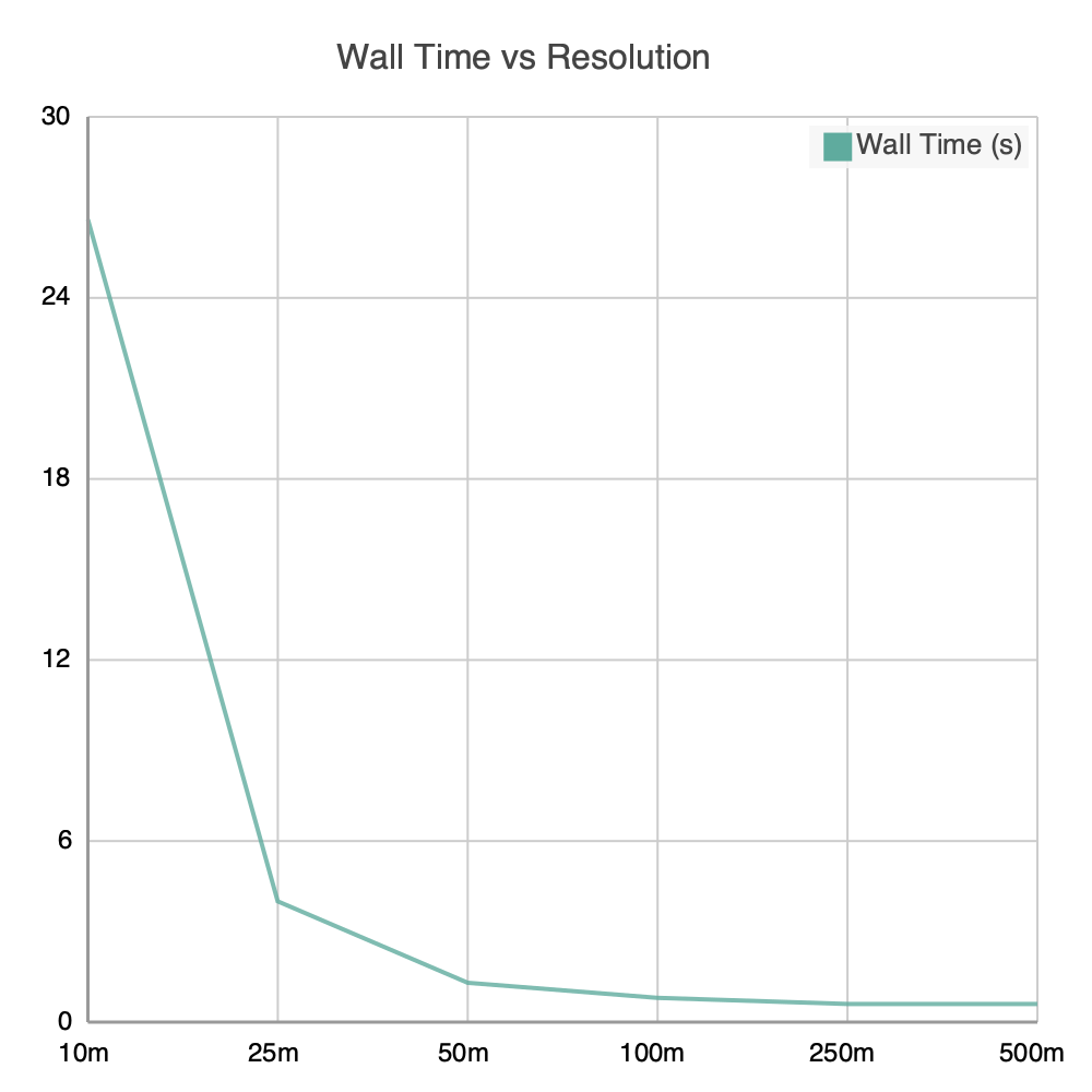
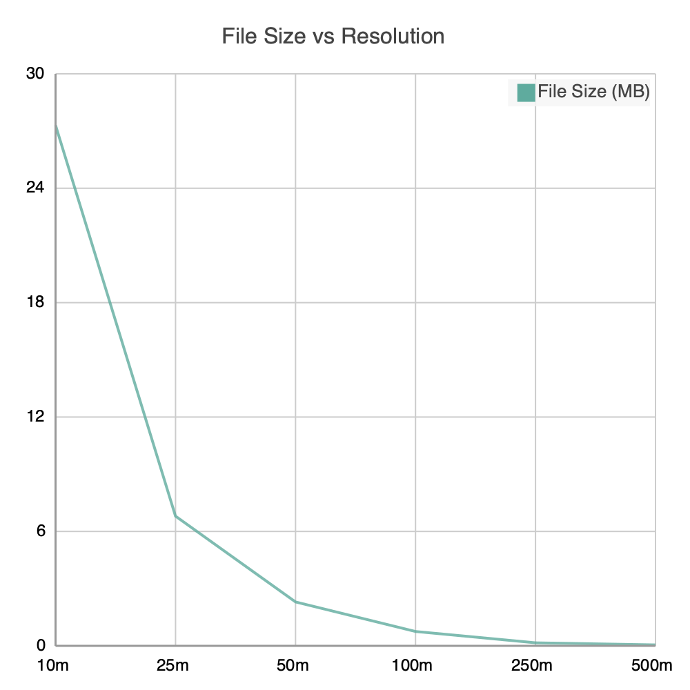
The tool was benchmarked using the Melbourne Housing dataset (13,580 points) at various resolutions on a single machine.
| Resolution | Wall Time | File Size |
|---|---|---|
| 10m | 26.6s | 27.3 MB |
| 25m | 4.0s | 6.8 MB |
| 50m | 1.3s | 2.3 MB |
| 100m | 0.8s | 749 KB |
| 250m | 0.6s | 159 KB |
| 500m | 0.6s | 49 KB |
Install
uv sync
Or manually:
pip install numpy pandas pyproj rasterio
Quick Start
# Interpolate Melbourne house prices
ppgrid data/melb_houses.csv --value-col price --res 500 --cap-km 10 --skip-calibration -o examples/melb/
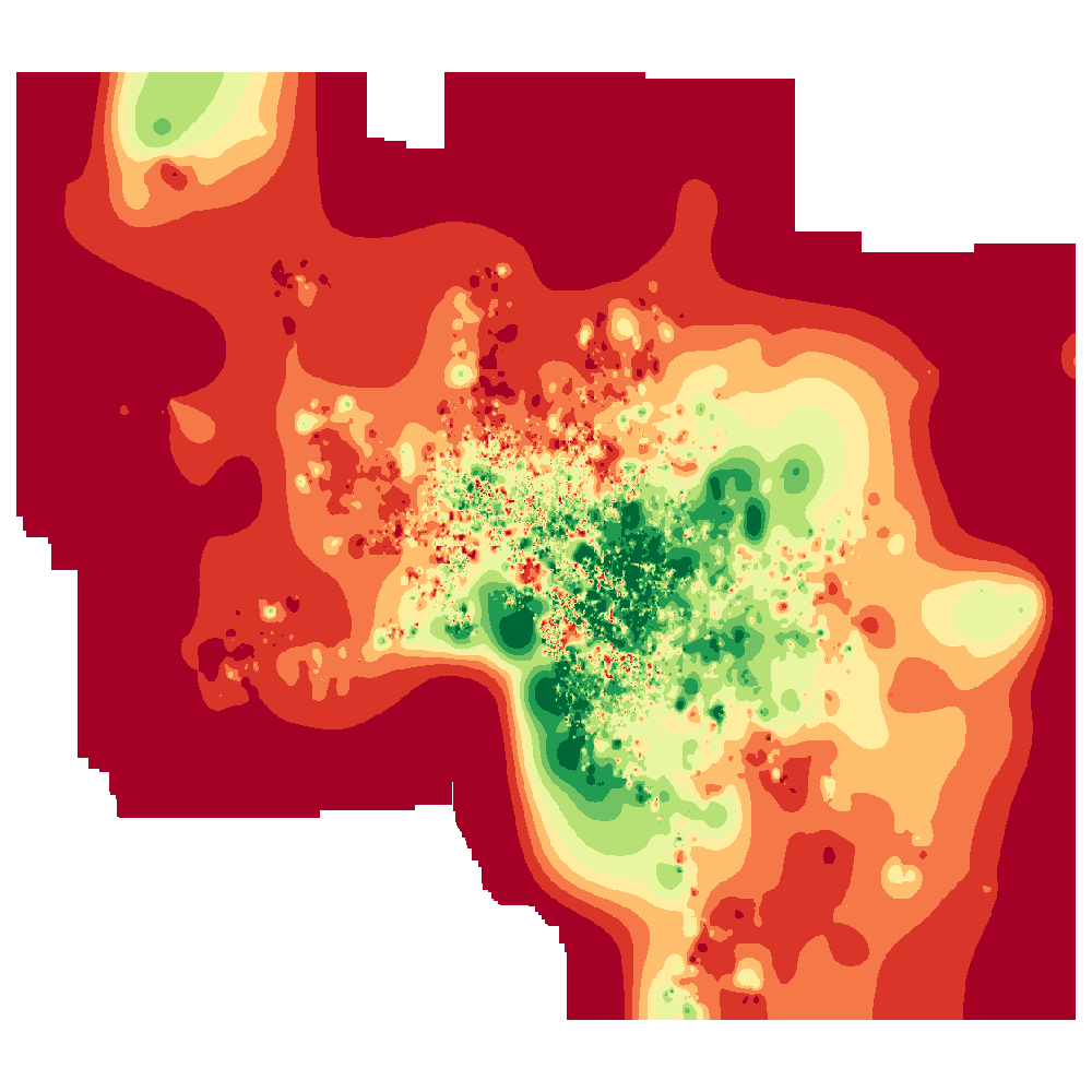
Example Outputs
The Melbourne Housing dataset (13,580 points) interpolated at 10m resolution:
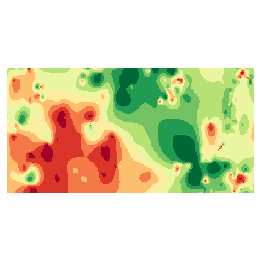
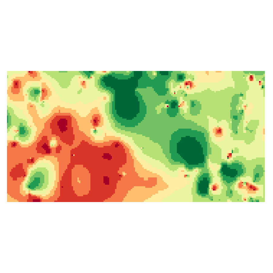
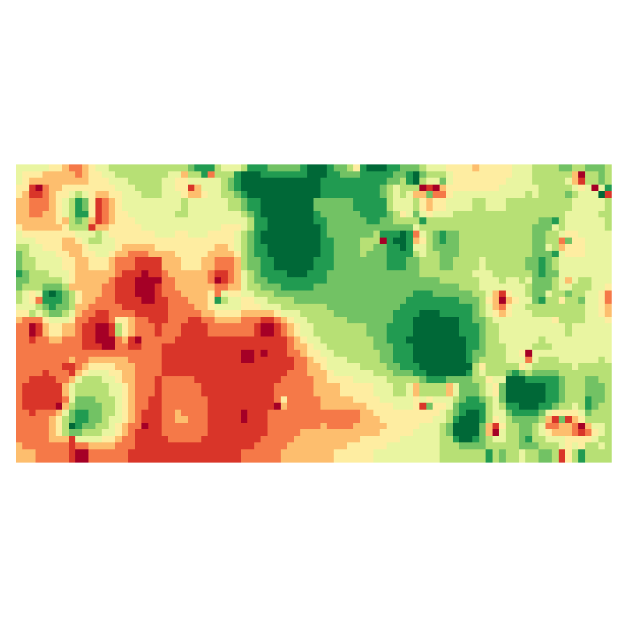
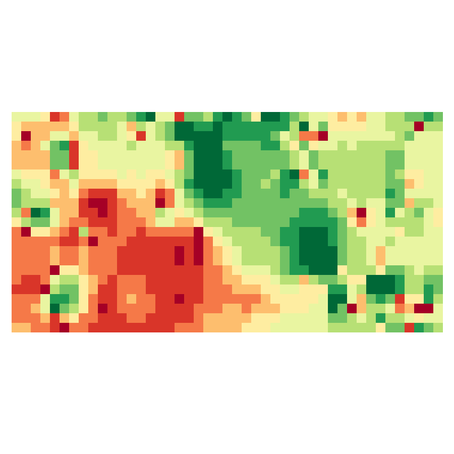
Cropped to the CBD to show resolution differences:
| 10m | 25m | 50m |
|---|---|---|
 |
 |
 |
| 100m | 250m | 500m |
|---|---|---|
 |
 |
 |
Usage
# Quick run (skip calibration)
python -m ppgrid data.csv --value-col premium --res 500 --cap-km 64 --skip-calibration

# Full run with calibration (saves calibration.json)
python -m ppgrid data.csv --value-col premium --res 100 --cap-km auto

# Custom projection and params
python -m ppgrid data.csv --value-col premium --res 100 --cap-km 25 --transform log10 --workers 8 --work-crs 3857 --out-crs 3857

# Reuse existing calibration
python -m ppgrid data.csv --value-col premium --calibration examples/previous/calibration.json
CLI Options
| Flag | Default | Description |
|---|---|---|
input |
(required) | CSV or Parquet input path |
-o, --out |
examples/ |
Output directory |
--value-col |
value |
Value column name |
--lng-col |
longitude |
Longitude column name |
--lat-col |
latitude |
Latitude column name |
--res |
500.0 |
Cell size in metres |
--cap-km |
auto |
Fill cap km, or 'auto' (blocked-CV derived) |
--transform |
auto |
auto | identity | log10 | sqrt | percentile |
--saturation |
1.0 |
Counts for a cell to fully self-trust |
--block |
8192 |
Block size in cells |
--workers |
4 |
Number of parallel workers |
--scale |
100.0 |
DN = percentile × scale |
--compress |
ZSTD |
GeoTIFF compression |
--calibration |
(none) | Path to existing calibration.json |
--calib-max-points |
2000000 |
Max points to use for calibration |
--src-crs |
4326 |
Input coordinate reference system |
--work-crs |
6933 |
Working CRS for interpolation (equal-area) |
--out-crs |
3857 |
Output CRS for final GeoTIFF |
--skip-calibration |
false | Skip calibration, use defaults |
Decoding the output
The value band stores percentiles, not raw values. To convert back to real units, use the calibration.json saved in the output folder:
import json, numpy as np, rasterio

with open("examples/test_run/calibration.json") as f:
    quantiles = np.array(json.load(f)["percentile_quantiles"])

with rasterio.open("examples/test_run/value.tif") as r:
    percentiles = np.array(r.read(1), copy=True) / 100.0

real_values = np.interp(percentiles, np.linspace(0, 100, len(quantiles)), quantiles)
Data
data/melb_houses.csv: 13,580 Melbourne property sales with latitude, longitude, and price. Sourced from the Melbourne Housing Snapshot (CC BY-NC-SA 4.0).
data/all_equakes.csv: 44,376 earthquake events from Jan–Aug 2026, mag ≥ 1.5.
Data Lineage
| Step | Description |
|---|---|
| Source | USGS Earthquake Hazards Program |
| API | FDSN Event Web Service |
| Download | Batched CSV requests by month, minmagnitude=1.5, starttime=2026-01-01, endtime=2026-08-08 |
| Processing | Concatenated monthly CSVs (deduplicated header) into single file |
| License | Public Domain (USGS federal data) |
Columns Used
latitude/longitude: spatial coordinates (WGS 84)mag: earthquake magnitude (continuous, for interpolation)depth: focal depth in km (optional value layer)time: event timestamp (ISO 8601)
1 maintainer

Download files
Download the file for your platform. If you're not sure which to choose, learn more about installing packages.
Source Distribution
Built Distribution
Filter files by name, interpreter, ABI, and platform.
If you're not sure about the file name format, learn more about wheel file names.
Copy a direct link to the current filters
File details
Details for the file ppgrid-0.1.1.tar.gz.
File metadata
- Download URL: ppgrid-0.1.1.tar.gz
- Upload date:
- Size: 86.8 MB
- Tags: Source
- Uploaded using Trusted Publishing? No
- Uploaded via:
uv/0.12.3 {"installer":{"name":"uv","version":"0.12.3","subcommand":["publish"]},"python":null,"implementation":{"name":null,"version":null},"distro":{"name":"Ubuntu","version":"24.04","id":"noble","libc":null},"system":{"name":null,"release":null},"cpu":null,"openssl_version":null,"setuptools_version":null,"rustc_version":null,"ci":true}
File hashes
| Algorithm | Hash digest | |
|---|---|---|
| SHA256 |
33ba5ce631f7e67a302ba42a38c6326b8877f77b47c46267cca9a7f17610b192
|
|
| MD5 |
e321b8982c53fc0598f6ac24ec0af976
|
|
| BLAKE2b-256 |
9f55d9ef67d8f1ccf4992ab1b8c7e9e79842d4cdab8e43b1a5b7c77e8ef9f525
|
File details
Details for the file ppgrid-0.1.1-py3-none-any.whl.
File metadata
- Download URL: ppgrid-0.1.1-py3-none-any.whl
- Upload date:
- Size: 19.9 kB
- Tags: Python 3
- Uploaded using Trusted Publishing? No
- Uploaded via:
uv/0.12.3 {"installer":{"name":"uv","version":"0.12.3","subcommand":["publish"]},"python":null,"implementation":{"name":null,"version":null},"distro":{"name":"Ubuntu","version":"24.04","id":"noble","libc":null},"system":{"name":null,"release":null},"cpu":null,"openssl_version":null,"setuptools_version":null,"rustc_version":null,"ci":true}
File hashes
| Algorithm | Hash digest | |
|---|---|---|
| SHA256 |
e595f006be2e1ae51d6839da1e9ceb02f41a143db83757c8595a679ae3c4e849
|
|
| MD5 |
3c3ffa9ccead813983dc9d3304e08976
|
|
| BLAKE2b-256 |
6350232170b36049fadf1246f3a5f3f95c42662e9c669744406c06eba54d55f5
|














