
PROSPECT, SAIL, PROSAIL, and GeoSail radiative transfer models

Project description
PROGEOSAIL Python Bindings
Valerio Pampanoni, mailto: valerio.pampanoni@uniroma1.it (Institutional), valerio.pampanoni@pm.me (Personal)
Repo Description
This is a fork of the jgomezdans/prosail Python bindings to the PROSPECT [1] and SAIL [2] leaf and canopy reflectance models. In addition to the features provided by the original code, I have ported over functions of Huemmrich's GeoSail model [3, 4], which exploits Jasinski's geometric model [5] to represent discontinuous vegetation canopies. The geocone and geocyli functions are available to model cone-shaped and cylindrical trees respectively. The legacy spelling geocily is also exported as an alias.
The default spectrum supported by this module falls between 400 and 2500 nm, with a spacing of 1 nm.
The bindings implement the following models:
- PROSPECT: versions 5 [6] and D [7]. Flexibility to add/modify leaf absorption profiles.
- SAIL: FourSAIL [8] version. The thermal extension of the model is also implemented, although this hasn't been widely tested.
- GEO: GEO part of Huemmrich's GeoSail code.
- Simple Lambertian soil reflectance model
Furthermore, I have completely re-written the parameter boundaries, and refer you to paragraphs 3.1.1, 3.1.2 and 3.1.3 of my PhD thesis for a detailed explanation of the meaning of each PROSPECT-D, 4SAIL and GEO variable respectively. The values are mostly sourced from [12], but you can find similar values in [13]. At the end of the README you can also find a small bibliography regarding the radiative transfer models, and another section about their usage for Live Fuel Moisture Content estimation.
Using the bindings
Import the bindings into the namespace with
import progeosail
If the import was successful, you may choose to run PROSPECT and SAIL individually or to run their coupled version in one go. Keep in mind that should you choose to run SAIL individually, you will have to provide your own leaf reflectance and transmittance spectra arrays, while using PROSPECT will allow you to generate them by setting the model parameters appropriately.
The progeosail module contains the following functions:
run_prospectrun_sailrun_prosailrun_progeosailgeoconegeocyligeocily, a backwards-compatible alias ofgeocyli
We will now go through each function individually.
The PROSPECT Model and the run_prospect Function
PROSPECT returns leaf reflectance and transmittance based on the biochemical characteristics of the leaf. Many different PROSPECT versions have surfaced since the publication of the original model in 1990, often introducing new parameters in the form of pigments. This implies that different model versions may require different parameters in order to run, and this module allows to choose between PROSPECT-5 and PROSPECT-D, which is used by default. The "D" in PROSPECT-D stands for "Dynamic", which refers to its capability to reproduce leaf phenology thanks to the addition of the anthocyanin pigment among the model variables. The complete list of PROSPECT-D model variables is summarized in the following table:
| Parameter | Description of parameter | Units | Typical min | Typical max |
|---|---|---|---|---|
| N | Leaf structure parameter | - | 1.0 | 3.0 |
| cab | Chlorophyll a+b concentration | ug/cm2 | 0 | 100 |
| caw | Equivalent water thickness | cm | 0.0001 | 0.0360 |
| car | Carotenoid concentration | ug/cm2 | 0 | 10 |
| ant | Anthocyanin concentration | ug/cm2 | 0 | 40 |
| cbrown | Brown pigment | - | 0 | 1 |
| cm | Dry matter content | g/cm2 | 0.0017 | 0.0960 |
In order to run PROSPECT-D we will have to call the run_prospect function and supply the anthocyanin pigment concentration (ant) as a keyword argument in addition to the leaf structure parameter (n), chlorophyll a and b concentration (cab), carotenoid pigment concentration (car), brown pigment (cbrown), water thickness (cw) and dry matter content (cm) as positional arguments:
wv, rho, tau = progeosail.run_prospect(n, cab, car, cbrown, cw, cm, ant=8.0)
Where rho and tau represent the , leaf reflectance and transmittance spectra respectively, and wv the wavelengths at which they were calculated.
In order to run PROSPECT-5, the prospect_version keyword argument must be supplied and must be set to '5', while there is no need to supply the anthocyanin content, since it is not included in the model:
lam, rho, tau = progeosail.run_prospect(n, cab, car, cbrown, cw, cm, prospect_version='5')
The SAIL Model and the run_sail Function
The Scattering by Arbitrarily Inclined Leaves (SAIL) model is one of the most widely used canopy reflectance models, and it was developed as an extension to Suits' 1972 one-dimensional, non-lambertian directional reflectance model [9]. In 1984, Verhoef proposed a novel solution of Suits' equations, introducing the Leaf Inclination Distribution Function (LIDF) in order to improve the model performance against changing illumination and viewing angles.
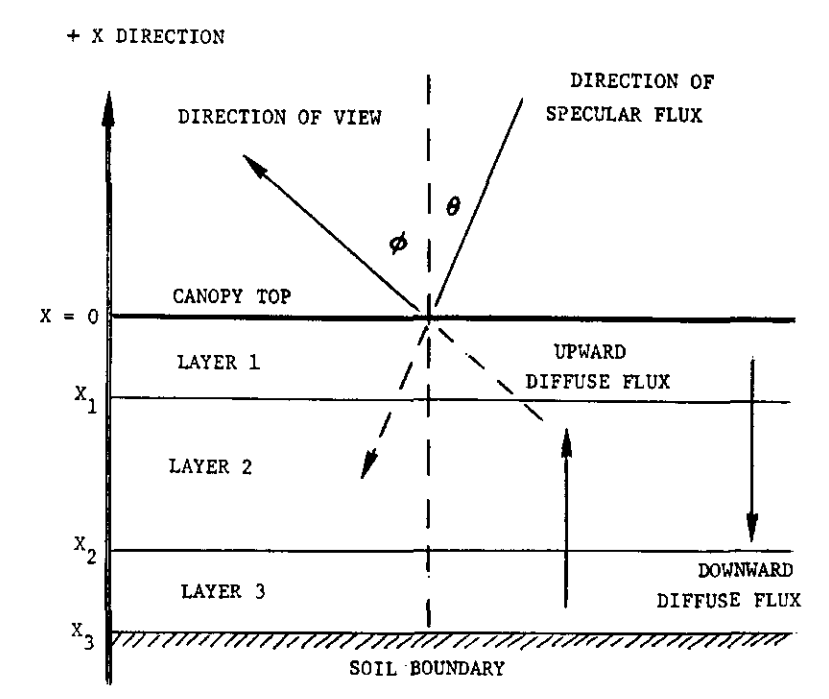
Figure 1: Suits' canopy model
An example of Suits' model is shown in the previous figure: each canopy layer (e.g. grain, stalk, leaves) is modeled as a horizontal, infinitely extended layer, and in turn each layer is composed of randomly distributed and homogeneously mixed components. The parameters of the SAIL model are summarized in the following table:
| Parameter | Description of parameter | Units | Typical min | Typical max |
|---|---|---|---|---|
| lai | Leaf Area Index | - | 0 | 7 |
| lidfa | Average Leaf Slope (Angle) | - (deg) | - | - |
| lidfb | Distribution bi-modality | - | - | - |
| psoil | Dry/Wet soil factor | - | 0 | 1 |
| rsoil | Soil brightness factor | - | 0 | 1 |
| hspot | Hotspot parameter | - | 0.01 | 0.40 |
| tts | Solar zenith angle | deg | 0 | 90 |
| tto | Observer zenith angle | deg | 0 | 90 |
| phi | Relative azimuth angle | deg | 0 | 360 |
| typelidf | Leaf angle distribution type | Integer | - | - |
In addition to the Leaf Area Index (LAI) and the hotspot factor (hspot), SAIL requires the user to define a number of parameters related to the inclination of the leaves that compose the canopy, the soil reflectance spectrum, and the solar and viewing illumination angles. In order to avoid confusion and to explain the ways these parameters can be supplied using this module, it is worth dedicating a small paragraph to each of them.
The Soil Spectra
As anticipated, SAIL requires the user to supply a soil reflectance spectrum in order to run. This module offers two pre-loaded soil spectra, rsoil1 which represents a dry soil, and rsoil2 which represents a wet soil. The numpy arrays containing the reflectance spectra can be accessed through the spectral_lib module as follows:
soil_spectrum1 = spectral_lib.soil.rsoil1
soil_spectrum2 = spectral_lib.soil.rsoil2
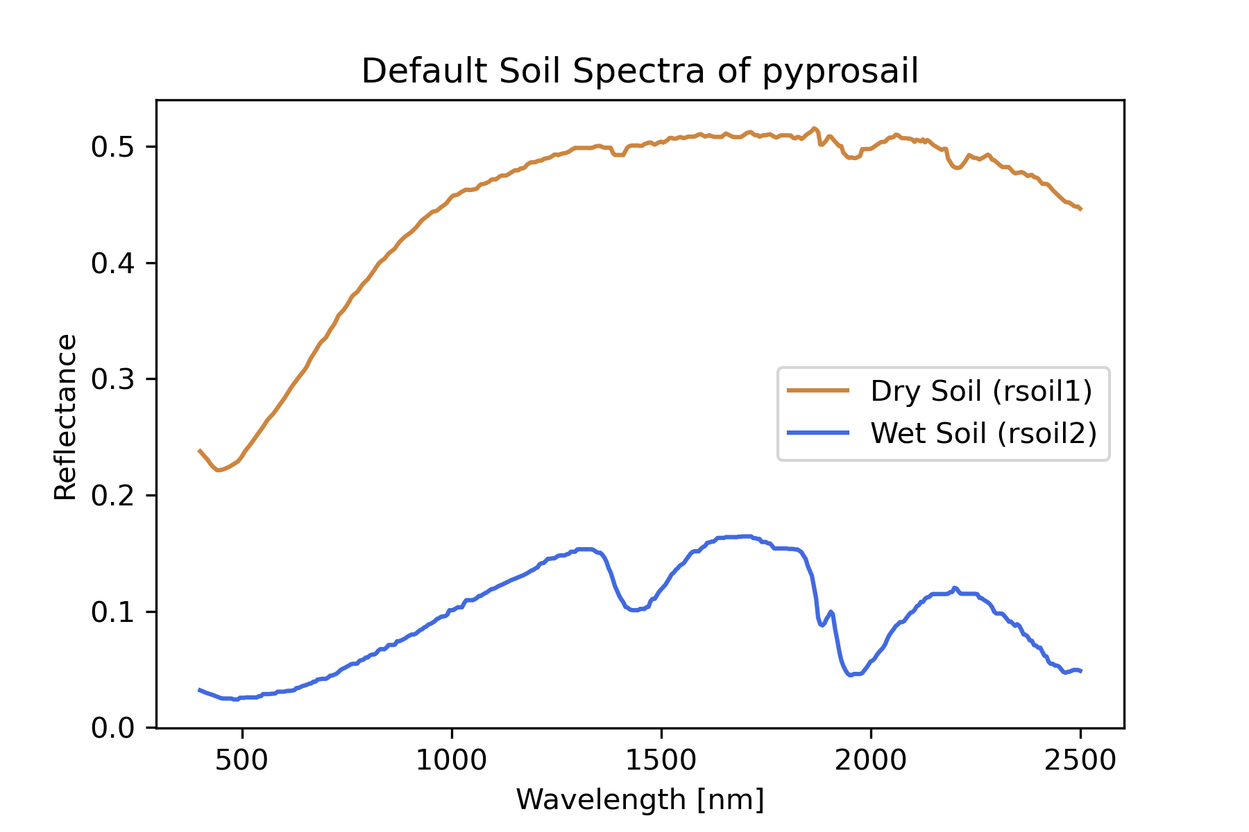
Figure 2: Default pyprosail soil spectra
Through the psoil and rsoil parameters allow the user to mix these two spectra in controlled proportions, using the following linear mixture model, where two spectra are mixed and then a brightness term added:
rho_soil = rsoil*(psoil*soil_spectrum1 + (1-psoil)*soil_spectrum2)
psoil can be considered a "soil dryness parameter", as values close to zero will return a soil reflectance spectrum dominated by the wet soil, while values close to one will return a soil reflectance spectrum dominated by the dry soil. rsoil acts as a generic soil brightness parameter, which we may use to scale the soil reflectance values.
The user may therefore use the two parameters psoil and rsoil to mix the default spectra as shown earlier. In addition, the user may supply an entirely new soil spectrum using the rsoil0 positional argument. Needless to say, if rsoil0 is supplied, the run_sail function will ignore psoil and rsoil if they were supplied. If no rsoil0 was supplied and only one of the psoil and rsoil parameters was supplied, the the run_sail function will throw an error.
The Leaf Inclination Distribution Function
The Leaf Inclination Distribution Function (LIDF) is used to represent in a simple way a number of different leaf orientations. Verhoef [10] described a method
to define a number of different LIDFs using two parameters: average leaf slope LIDFa, and distribution bi-modality LIDFb. In addition to this method of LIDF representation, this library allows to use a simple ellipsoidal function characterized by a singular parameter representing the average leaf inclination angle.
The parameter typelidf allows to switch between one method and the other:
typelidf = 1: use the Verhoef two-parameter method, whereLIDFaandLIDFbcontrol the average leaf slope and the distribution bimodality, respectively. Popular distributions are given by the following parameter combinations:
| LIDF type | LIDFa |
LIDFb |
|---|---|---|
| Planophile | 1 | 0 |
| Erectophile | -1 | 0 |
| Plagiophile | 0 | -1 |
| Extremophile | 0 | 1 |
| Spherical | -0.35 | -0.15 |
| Uniform | 0 | 0 |
typelidf = 2Campbell distribution, whereLIDFaparameter represents the average leaf angle (0 degrees is planophile, 90 degrees is erectophile). In this case, theLIDFbparameter is ignored.
By default, the run_sail function expects typelidf = 2, and therefore only the LIDFa value is required to run it. If the user wants to use the Verhoef parametrization, typelidf should be set to 1, and both LIDFa and LIDFb should be supplied.
Solar and Viewing Angles
A graphical representation of the Sun-Sensor geometry is shown in the following figure:
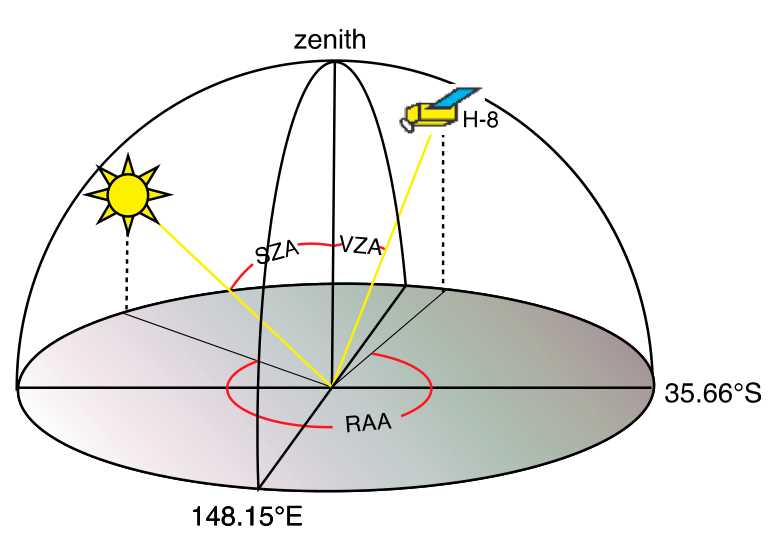
Figure 3: Sun-Sensor geometry scheme
SAIL expects the user to set the following three angular parameters:
- The Solar Zenith Angle (SZA)
tts - The Viewer Zenith Angle (VZA)
tt0 - The Relative Azimuth Angle (RAA)
phi, defined as the difference between the Solar Azimuth Angle (SAA) and the Viewer Azimuth Angle (VAA)
Running SAIL
To run SAIL with two one-dimensional arrays of leaf reflectance and transmittance sampled with a 1 nm spacing between 400 and 2500 nm rho and tau, using an ideal black soil (e.g. zero reflectance), we can use the following command:
rho_canopy = progeosail.run_sail(rho, tau, lai, lidfa, hspot, sza, vza, raa, rsoil0=np.zeros(2101))
As explained in the previous sections, the user may:
-
use a Verhoef-style two-parameter LIDF:
rho_canopy = progeosail.run_sail(rho, tau, lai, lidfa, hspot, sza, vza, raa, lidftype=1, lidfb=lidfb, rsoil0=np.zeros(2101)) -
use
psoilandrsoilto mix the default spectra:rho_canopy = progeosail.run_sail(rho, tau, lai, lidfa, hspot, sza, vza, raa, lidftype=1, lidfb=lidfb, rsoil=rsoil, psoil=psoil) -
re-assign the
soil_spectrum1andsoil_spectrum2keywords to supply custom soil spectra and mix them using thepsoilandrsoilkeywords:rho_canopy = progeosail.run_sail(rho, tau, lai, lidfa, hspot, sza, vza, raa, lidftype=1, lidfb=lidfb, rsoil, psoil, soil_spectrum1=custom_soil1, soil_spectrum2=custom_soil2)
By default, run_sail returns the surface directional reflectance (SDR), but you can choose other reflectance factors by setting using the factor keyword argument to the appropriate value:
factor |
Description |
|---|---|
| SDR | Surface Directional Reflectance factor |
| BHR | Bi-Hemispherical Reflectance factor |
| DHR | Directional-Hemispherical Reflectance factor |
| HDR | Hemispherical-Directional Reflectance factor |
| ALL | All of the above |
| ALLALL | All of the terms calculated by SAIL, including the above |
PROSPECT + SAIL and the run_prosail Function
As anticipated, PROSPECT's output in terms of leaf reflectance and transmittance spectra can be directly fed into SAIL as an input. The inversion of PROSPECT is relatively easy, but from a remote sensing point of view, inverting the reflectance spectra of a singular leaf has limited applicability. On the other hand, SAIL provides a description of a leaf canopy, but its inversion from satellite or airborne data can be feasible only when several measurements from different viewing angles are available, which is almost never the case. To solve this issue, the two models were coupled into PROSAIL [73] since the early nineties. A graphical representation of the coupling scheme is shown in Figure 4.
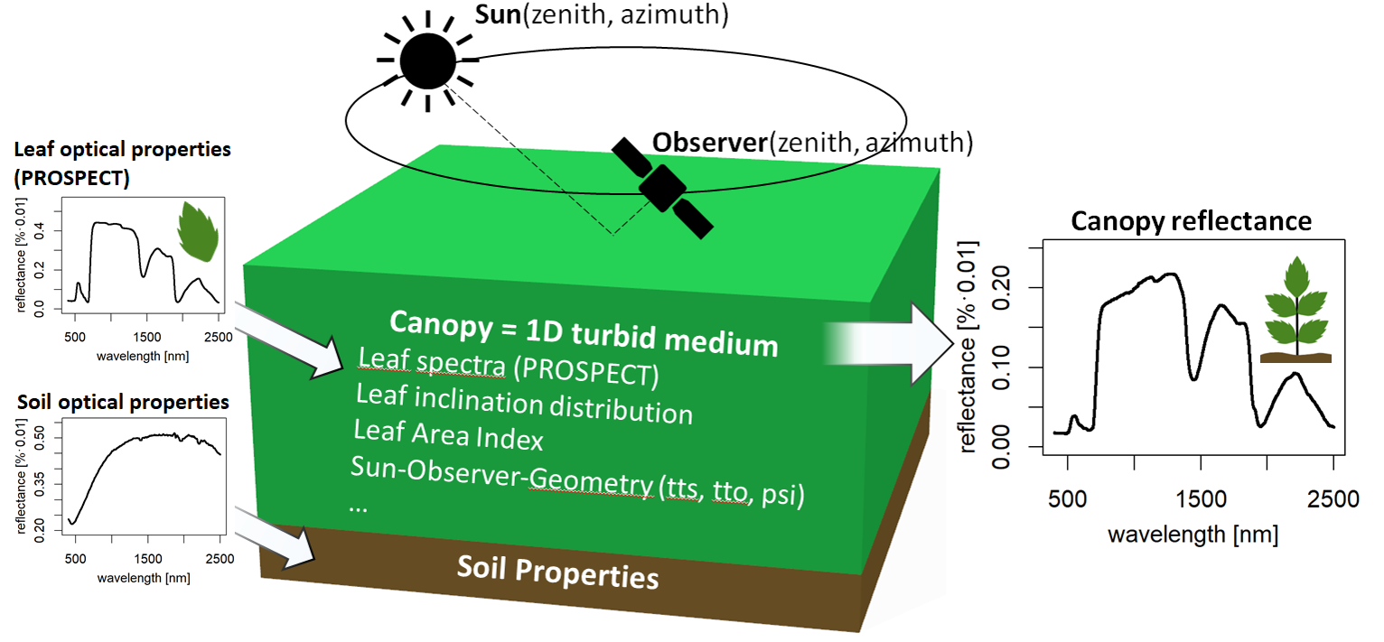
Figure 4: PROSPECT + SAIL Coupling Scheme
The run_prosail function can be used to run the combination of PROSPECT-5 or PROSPECT-D and SAIL in one step:
rho_canopy = progeosail.run_prosail(n, cab, car, cbrown, cw, cm, lai, lidfa, hspot, tts, tto, psi)
ProGeoSail and the run_progeosail Function
In 2001 [3], the SAIL model was coupled with the Jasinski Geometric model (GEO) with the objective to allow the description of radiation reflected by and transmitted through discontinuous vegetation. In order to port this functionality to pyprosail, we rewrote the Fortran subroutines GEOCONE and GEOCYLI to Python, and interfaced them with the existing PROSAIL functions. At the moment, only nadir view is supported, and for this reason only the Sun Zenith Angle is included in the input variables, while the Viewing Zenith Angle is assumed to be zero.
| Parameter | Description | Units |
|---|---|---|
tts |
Sun Zenith Angle | deg |
rc |
Nadir-view reflectance of illuminated canopy | - |
tc |
Transmittance through canopy | - |
rch |
Hemispheric reflectance through canopy | - |
chw |
Canopy height-to-width ratio | m/m |
ccover |
Fraction of Canopy Cover | m^2/m^2 |
cshp |
Crown Shape | - |
The reflectance and transmittance spectra are all supplied by SAIL. If the Observer Zenith Angle tto is set to zero (nadir view), the hemispherical-directional reflectance and transmittance through the canopy will correspond to rc and tc respectively, while the bi-hemispherical reflectance factor will correspond to rch. The cshp parameter allows to set the tree shape among the two currently supported, which are 'cylinder' and 'cone'. More can be implemented following the methodology described in [5].
A minimal run_progeosail run would look like this:
rsc, gsfr = progeosail.run_progeosail(chw, ccover, cshp,
                                      n, cab, car, cbrown, cw, cm,
                                      lai, lidfa, hspot, tts, tto, psi)
run_progeosail returns a tuple (rsc, gsfr), where rsc is the scene reflectance spectrum and gsfr is Huemmrich's instantaneous fraction of absorbed radiation. When the input band corresponds to PAR wavelengths, gsfr can be interpreted as FAPAR.
The two geometric GeoSail functions can also be used directly if the crown optical properties have already been calculated. Both functions return the same (rsc, gsfr) tuple:
rsc, gsfr = progeosail.geocone(chw, ccover, tts, rc, tc, rch, rsoil0)
rsc, gsfr = progeosail.geocyli(chw, ccover, tts, rc, tc, rch, rsoil0)
where rc is the nadir-view crown reflectance, tc is the crown transmittance, rch is the hemispherical crown reflectance, and rsoil0 is the background reflectance. rsc and gsfr can be scalars or spectra, depending on whether scalar reflectance values or wavelength arrays are supplied.
Bibliography
Figure References
Figure 1: [9]
Release history Release notifications | RSS feed

Download files
Download the file for your platform. If you're not sure which to choose, learn more about installing packages.
Source Distribution
Built Distribution
Filter files by name, interpreter, ABI, and platform.
If you're not sure about the file name format, learn more about wheel file names.
Copy a direct link to the current filters
File details
Details for the file progeosail-2.1.0.tar.gz.
File metadata
- Download URL: progeosail-2.1.0.tar.gz
- Upload date:
- Size: 205.4 kB
- Tags: Source
- Uploaded using Trusted Publishing? No
- Uploaded via: twine/6.2.0 CPython/3.12.13
File hashes
| Algorithm | Hash digest | |
|---|---|---|
| SHA256 |
76835fc7ae08b2b0d0fd9ec12a4974efe757126fd7152795809a3b0ddfb36364
|
|
| MD5 |
2a558a5b845a55e3c19929c9a9b7f289
|
|
| BLAKE2b-256 |
ecb613ecea2da5e26722544f88e88b1a4e4eda77551218f69a5abeb9593ed7df
|
File details
Details for the file progeosail-2.1.0-py3-none-any.whl.
File metadata
- Download URL: progeosail-2.1.0-py3-none-any.whl
- Upload date:
- Size: 198.8 kB
- Tags: Python 3
- Uploaded using Trusted Publishing? No
- Uploaded via: twine/6.2.0 CPython/3.12.13
File hashes
| Algorithm | Hash digest | |
|---|---|---|
| SHA256 |
05688a4ca33762acaa571adc0f358937c21e4dc75568da876aaefa94ee84e4bf
|
|
| MD5 |
9a209c7fc24a6b81c28810af3c0dc203
|
|
| BLAKE2b-256 |
8a880a724a91a9f965bccf16827a76806cb137933ddf5d2d62fcba8cf83acb08
|






