
Interactive data exploration workbench for local CSV files, Parquet files, and same-schema Parquet folders.
Verified details
These details have been verified by PyPIProject links
GitHub Statistics
Maintainers

Project description
lucidum
lucidum is a local browser workbench for exploring CSV and Parquet datasets. It starts a small local FastAPI server, reads data with DuckDB, and opens an interactive UI for profiling columns, plotting grouped metrics, applying filters, and mapping UK postcode data.
The app is designed for local analysis: your dataset stays on the machine running lucidum.
Current Tools
-
Dataset Viewer: inspect a fast filtered preview of dataset rows in a sortable Tabulator grid, capped at 100 displayed rows, with client-side whole-table search, axis-exclusive whole-row or whole-column selection, transpose mode where search matches original column-name rows while keeping all preview row columns, optional alphabetical column ordering, right-click column pinning that marks pinned names, lists pinned columns above the grid, and keeps pinned columns first and visible during column search without frozen or sticky cells, saved Dataset view favourites including sort state, right-click cell copy, and right-click CSV copy for selected rows or columns.
-
Column Profile: review dataset columns, missing values, distinct counts, ranges, value counts, and numeric/date distributions. Logical/boolean columns are labelled
logicalwhile retaining categorical analysis behavior. Large datasets open with a fast preview summary and can be recalculated on all rows. Right-click a column row to copy the feature name. -
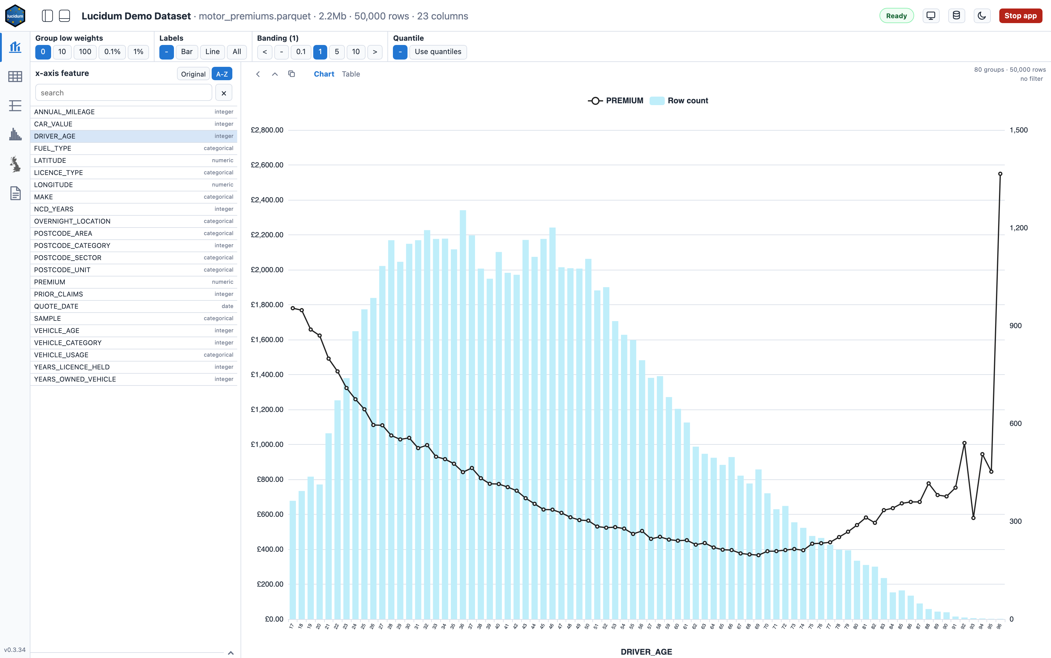
Line and Bar: plot grouped Actual and up to two optional Expected response values over one or two features in a full-bleed chart/table workspace. Its scrollbar-free settings strip uses edge fades to mark off-screen controls and supports horizontal trackpad/touch gestures, keyboard focus scrolling, and ordinary vertical mouse-wheel scrolling. One-feature views retain the existing line/bar controls, including sorting, transforms, sigma bars, SHAP ribbons, and GLM partial-dependence overlays. A plain feature click always makes that row the sole Feature 1; Command-click another feature on macOS, or Ctrl-click it on Windows/Linux, to add or remove Feature 2 without disabling the remaining rows. The double-ended arrow beside the x-axis heading swaps the two features together with their independent grouping controls in one refresh. Two untreated continuous numeric/date groupings render a surface whose axes use the exact plotted data ranges and whose 3D footprint expands responsively on wider chart areas, continuous/factor groupings render colour-matched response lines with stacked Weight/N bars, and factor/factor groupings render a heatmap whose category axes independently suppress tick labels that cannot fit at the 8px legibility floor while retaining axis titles and tooltips. Dates are continuous by default, use chronological date-aware line/surface axes, and expose
Treat as factoralongside their independent calendar bucket so the same pair can switch to lines or a heatmap. Numeric features expose the same override alongside independent banding and quantile controls. A one-featureMissings — Show / Hidecontrol, or one independent control per feature in two-feature mode, either retains missing groups or removes raw rows missing that feature from the Line/Bar analysis. Shown missing-volume bars use pale grey. Hide recalculates the Line/Bar chart, table totals, transforms, overlays, pagination, and displayed Line/Bar row count, but the shared sidebar Numerator and Denominator values remain based on the global filter so switching tools does not change their meaning. Numeric tails Winsorise fixed-width values at that feature's percentile cutoffs; categorical tails combine at least two marginal levels at or below the chosen share of filtered Weight/N intoOther. In one-feature ordered low-weight grouping, shown missings stay separate and do not consume either tail, although percentage thresholds still use total included Weight/N. Quantile, date, and unbanded numeric groupings ignore two-feature Tail grouping. Mixed line/bar plots always show volume and offer a cached Plot chooser only when multiple response values are available; surfaces and heatmaps show one chosen response or Weight/N at a time. Factor/factor heatmaps accept up to 100,000 populated grouped cells; other Line/Bar charts retain the 10,000-group guard. Heatmaps offer cached-,Actual,Weight, and, where two lines fit,Bothcell labels, using active-KPI response formatting, contrast-aware text colours, and responsive font sizing. Each label mode remains available at larger category counts whenever its formatted text still fits at the separate 7px cell-label floor. The server-backed table keeps both feature columns and every selected response. The tool also supports a shared Denominator, including the active primary GLM or GBM prediction joined by row identity, lazily estimated numeric banding, date buckets with optional empty-period display in one-feature mode, searchable/paginated tables, A-Z picker defaults, a launch-collapsed Expected picker, saved Favourites views, an active GBM/GLM prediction-ratio feature, and feature ordering by saved GBM/GLM importance. -
Histogram: plot the selected Actual value, or Actual divided by Weight, as a filtered distribution in a full-bleed workspace with a launch-collapsed borderless settings strip and a compact metrics table separated from the chart by a draggable divider. When a Denominator is selected, the x-axis title identifies the plotted calculation as
Numerator / Denominator; Average row value shows only the Numerator. Histogram supports bin counts or explicit original-unit bin widths with boundaries anchored to rounded width multiples, integer-aware bins for discrete numeric Actuals, optional responsive values above bins, denser fit-aware x-axis labels, sampled 100k previews or exact all-row mode, cumulative/probability modes, log axes, mean/median reference lines, and saved Histogram view favourites. -
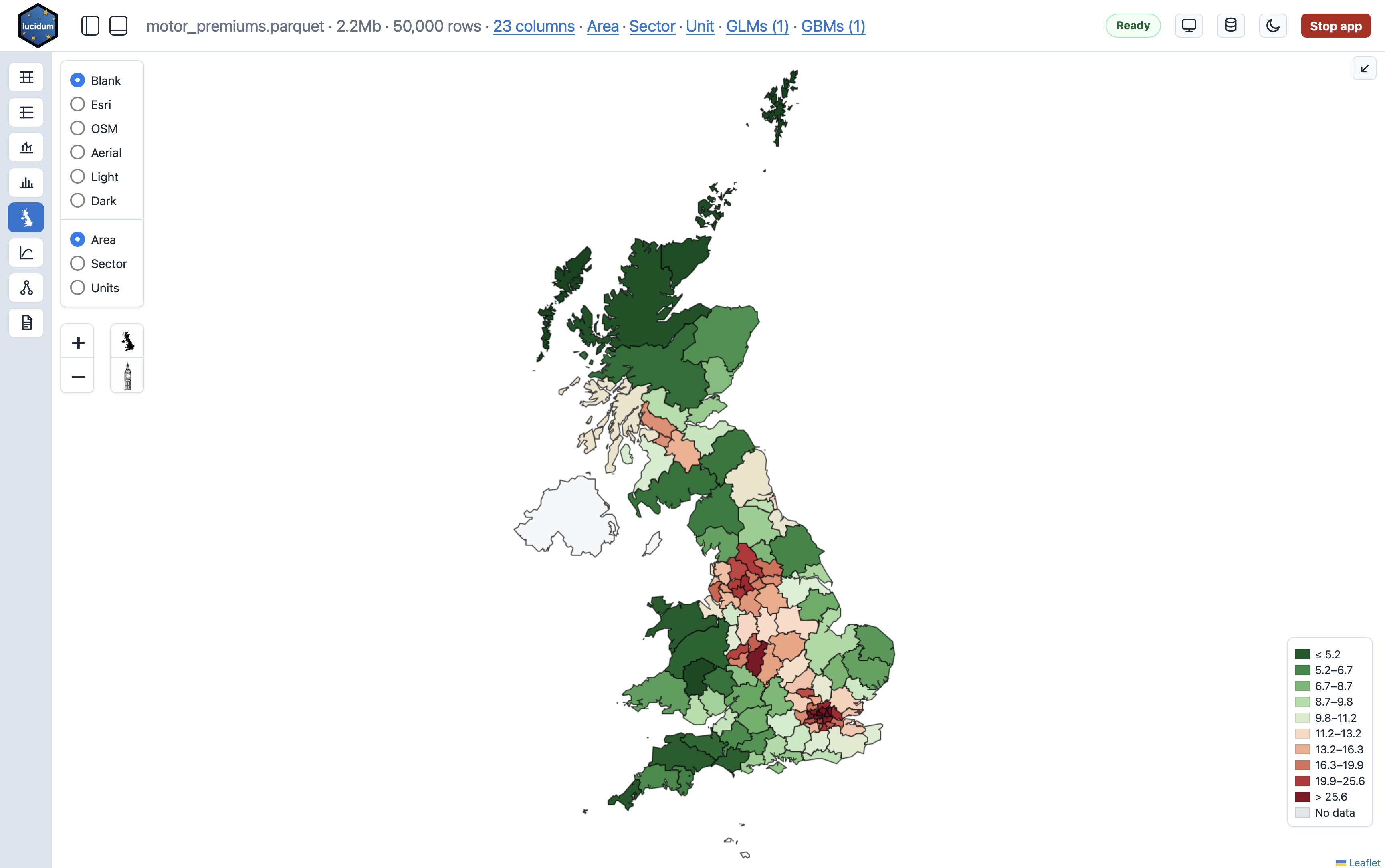
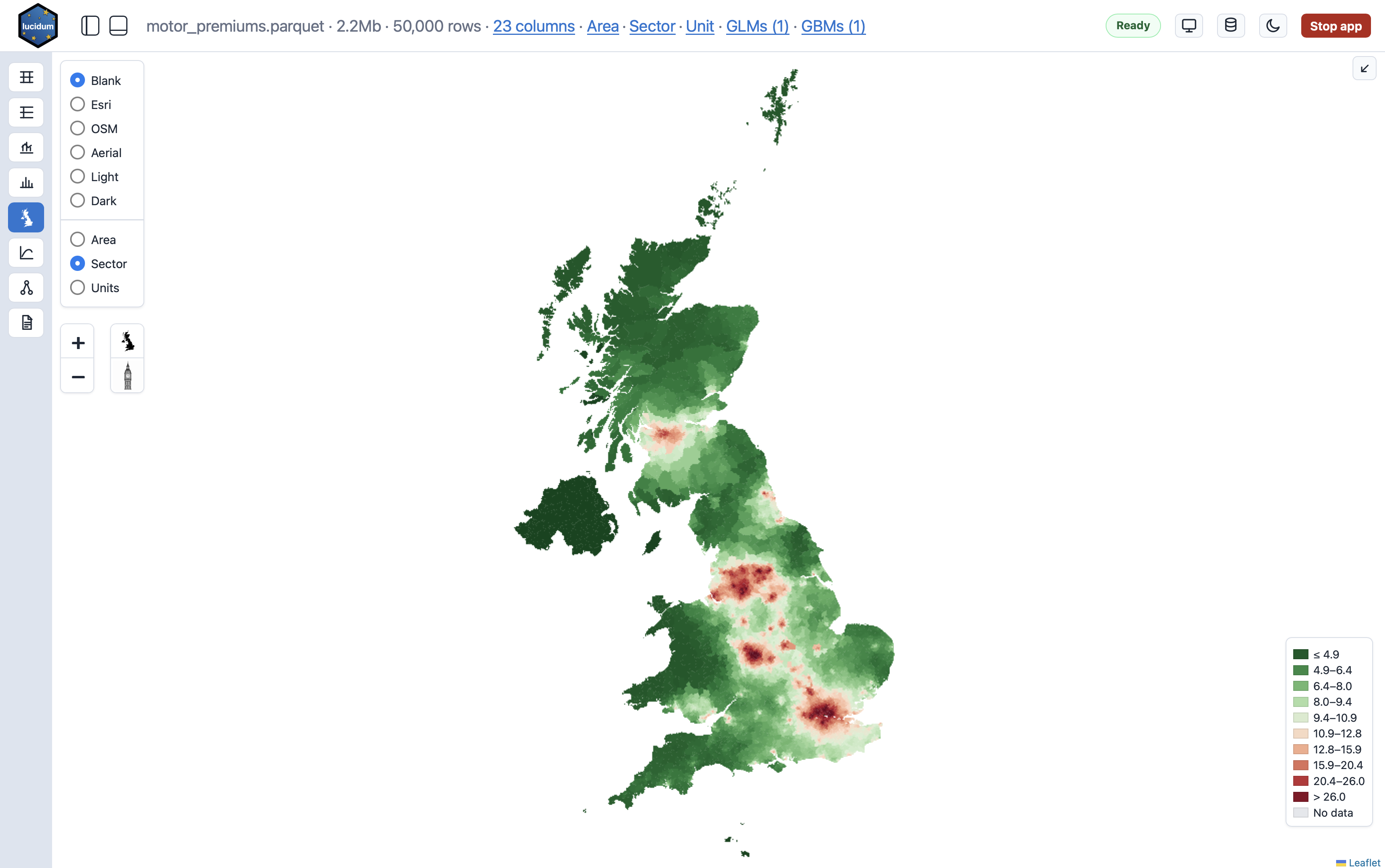
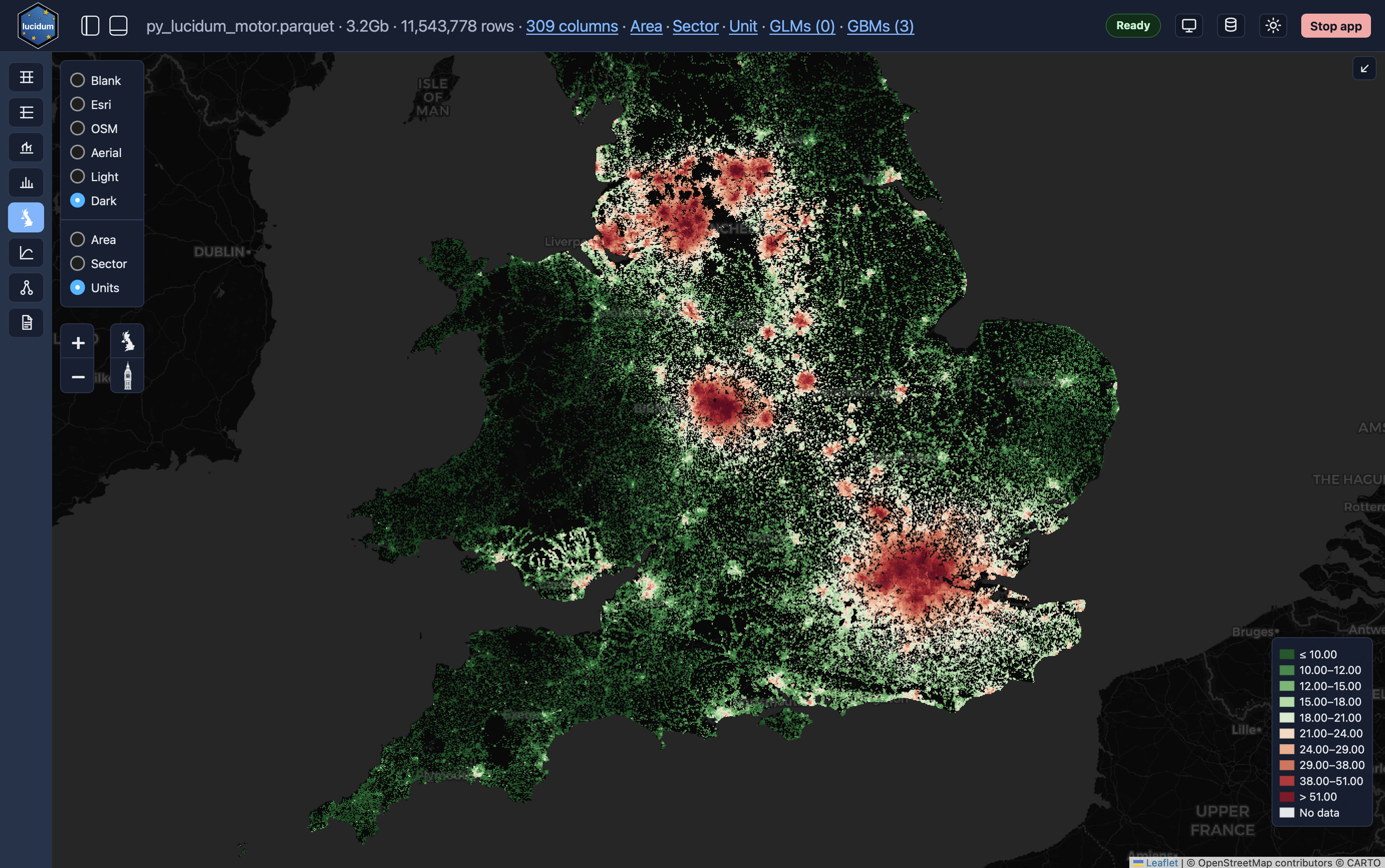
UK Mapping: map postcode areas and sectors with bundled GeoJSON, including optional sector neighbour smoothing, or postcode units when unit and coordinate columns are available. Area and sector maps continue plotting valid geometry when some nonblank postcode values are absent from the bundled shapes, report the affected row count and percentage below the geometry match count, and report blank postcode counts and percentages separately. Colour legends and hotspot selection use only values attached to geometry that can actually be drawn. The floating map panel shows the wrapped KPI name when the selected Numerator and Denominator match a KPI, and omits the heading when they do not. Right-click the map at any resolution to stage a postcode-region selection and apply it as one global area filter; postcode popups provide View rows, Zoom, Copy, and postcode filtering actions.
-
GLM: optional
glummodel building with Formulaic formulas, coefficient tables, persisted tabulations/rating tables with XLSX export, and activeglm_prediction, denominator-backedglm_prediction_rate, andglm_tabulated_predictionsources that can be plotted like other model predictions. The header status badge reports elapsed time from the build click through fitting and post-fit scoring, and separately times tabulation through row scoring. -
GBM: optional LightGBM model building with persistent sidecar artifacts, predictions and denominator-backed prediction rates that can be plotted as chart/map data sources, evaluation plots, model navigation, tree viewing, SHAP plotting when SHAP rows are saved during training, and XLSX export for saved tabulations. The header status badge reports elapsed time through training, scoring, SHAP calculation, artifact saving, and final client refresh.
-
Filters, Favourites, KPIs, and Feature specs: apply free-form DuckDB
WHEREfilters, saved filter rows, sidebar Favourites for saved metric/filter/Line/Bar/Histogram/Map views, separate KPI metric presets, and GBM feature scenarios/interaction constraints. -
Specifications: default editor tab for feature, KPI, and filter specification CSV files, with continuous validation and save actions against the app's current metadata contracts.
The two shared metric headings in the sidebar are Numerator and Denominator; this is a presentation-only rename, so chart legends, tables, APIs, KPI files, and model metadata retain their existing Actual/Weight terminology. The Denominator selector groups numeric dataset columns separately from the active primary glm_prediction and gbm_prediction outputs. Activating a saved GLM or GBM, including automatic promotion after deleting the active model, atomically selects that model's saved training Numerator and Denominator before the visible chart refreshes. A selected model denominator follows the active model of that type, and Line/Bar, Histogram, UK Map, and sidebar summaries refresh against the replacement model. GLM and GBM building is disabled while a model prediction is the Denominator; prediction chaining remains available through GBM init_score.
Line/Bar response axes identify the selected calculation as Numerator / Denominator, using the underlying column names (for example, PREMIUM / glm_prediction). With Average row value, only the Numerator name is shown. Single-feature charts use the same convention for the primary Numerator legend entry while keeping Expected and Denominator entries unchanged. The secondary Denominator/row-count axis reserves space from its formatted tick widths so its labels remain clear of the vertical axis title.
Unreadable dataset columns, such as Parquet strings with invalid UTF-8, are skipped by the shared schema used by normal selectors. Column Profile reports them as skipped, and the GBM feature chooser shows them as disabled invalid rows.
Installation
Lucidum requires Python 3.13 or newer. Both pip and pipx download the same
py-lucidum package from PyPI. For a user-level lucidum command, pipx is
recommended because it gives Lucidum its own isolated environment and exposes
the command on your PATH. Choose the optional modelling extras you need at
install time:
pipx install --python python3.13 py-lucidum
pipx install --python python3.13 "py-lucidum[glm]"
pipx install --python python3.13 "py-lucidum[gbm]"
pipx install --python python3.13 "py-lucidum[glm,gbm]"
For a reproducible Lucidum version, pin the release explicitly:
pipx install --python python3.13 "py-lucidum==0.4.59"
pipx install --python python3.13 "py-lucidum[glm,gbm]==0.4.59"
The pip install py-lucidum command shown at the top of the PyPI project page
is also supported. pip installs into whichever Python environment is
currently selected, so on a clean machine create and activate a virtual
environment first. On macOS or Linux:
python3.13 -m venv lucidum-venv
source lucidum-venv/bin/activate
python -m pip install --upgrade pip
python -m pip install "py-lucidum==0.4.59"
On Windows PowerShell:
py -3.13 -m venv lucidum-venv
.\lucidum-venv\Scripts\Activate.ps1
python -m pip install --upgrade pip
python -m pip install "py-lucidum==0.4.59"
Omit ==0.4.59 to install the latest release. To include both optional
modelling toolsets with plain pip, use:
python -m pip install "py-lucidum[glm,gbm]==0.4.59"
Once the virtual environment is active, lucidum is available in that
terminal. Using python -m pip makes explicit which Python environment receives
the installation; do not use sudo pip for Lucidum.
Use the same requirement in another Python project's dependency metadata or requirements file:
py-lucidum==0.4.59
An exact Lucidum pin fixes Lucidum's code but does not pin DuckDB, FastAPI, or its other transitive dependencies. Use the consuming project's normal lock or constraints file when the complete environment must be reproducible.
On macOS, LightGBM also needs the OpenMP runtime. This applies whether you
install with a virtual environment or pipx. If training fails with a
libomp.dylib load error, install it with:
brew install libomp
Upgrade an existing PyPI installation with:
pipx upgrade py-lucidum
To change the installed extras, reinstall with the desired spec:
pipx uninstall py-lucidum
pipx install --python python3.13 "py-lucidum[glm,gbm]"
If PyPI is unavailable, install the same immutable release from its Git tag:
pipx install --python python3.13 "py-lucidum @ git+https://github.com/SpeckledJim2/py_lucidum.git@v0.4.59"
pipx install --python python3.13 "py-lucidum[glm,gbm] @ git+https://github.com/SpeckledJim2/py_lucidum.git@v0.4.59"
Quote package specifications containing extras exactly as shown, because shells
can interpret [glm,gbm] as a filename pattern. The distribution name used by
installers is py-lucidum, the Python import is py_lucidum, and the installed
command is lucidum.
For development from a source checkout, create an editable environment from the project root:
python3.13 -m venv .venv
.venv/bin/python -m pip install --upgrade pip
.venv/bin/python -m pip install -e .
.venv/bin/python -m pip install -e ".[glm]"
.venv/bin/python -m pip install -e ".[gbm]"
For a pipx command backed by a local checkout, use the same extra names with the local path:
pipx install --python python3.13 /path/to/py_lucidum
pipx install --python python3.13 "/path/to/py_lucidum[glm,gbm]"
Quick Start
Launch the bundled synthetic demo dataset:
lucidum --demo --port 8000
This command works after either the pipx installation or activation of the
plain-pip virtual environment. From a source checkout whose development
environment is not activated, use .venv/bin/lucidum instead. Open the printed
URL in your browser. Stop the server with Ctrl+C in the terminal. Pass
--buttons when you want the browser header to show Stop app and Open monitor buttons.
Demo launches label the header as Lucidum Demo Dataset · motor_premiums.parquet · ... before the size, row count, and column count.
The sidebar footer shows the installed Lucidum package version as lucidum v<version> when expanded and v<version> when collapsed. Both labels are populated from the running app's schema metadata.
Run your own data:
.venv/bin/lucidum path/to/my_data.parquet --port 8000
.venv/bin/lucidum path/to/my_data.csv --port 8000
.venv/bin/lucidum path/to/monthly_parquets/ --port 8000
From a source checkout, datasets/monthly/ contains a seven-file monthly split
of the demo data that exercises folder input:
.venv/bin/lucidum datasets/monthly --port 8000
If installed with pipx, use:
lucidum path/to/my_data.parquet --open
lucidum path/to/my_data.csv --open
lucidum path/to/my_data.parquet --tools line-bar,glm --open
lucidum path/to/my_data.parquet --tools line-bar,glm,gbm --open
Use --tools all after installing the needed modelling extras when you want to
load every available tool, including GLM and GBM.
Parquet is recommended for normal use because DuckDB can read it efficiently.
You can also pass a folder containing direct-child .parquet files. Lucidum
reads those files as one dataset when every file has identical column names and
DuckDB types. Non-Parquet files and nested folders are ignored. Folder inputs
are available only when GLM and GBM are not enabled; use a single Parquet file
for modelling tools. The app header displays folder inputs with their file
count, for example monthly (7 files).
Use --title-prefix to put your own text before the file or folder name,
separated by the same middle dot used by the rest of the header metadata.
Dataset Workspaces
Lucidum stores model sidecars beside the data folder under a hidden dataset-scoped workspace:
.lucidum/datasets/<dataset-slug>/<dataset-signature>/models/
The dataset slug comes from the CSV or Parquet filename. The dataset signature is based on the file size, modification time, row count, and schema fingerprint. This means one folder can safely contain many datasets: models trained for one file do not attach to another file in the same folder.
If a dataset file is replaced or edited, it gets a new signature workspace. Existing GLM/GBM models from the previous version remain on disk but are not shown or used; rebuild models after changing the source file. Older root-level .lucidum/models/ folders are ignored by current Lucidum versions. Parquet folder inputs do not create or read GLM/GBM workspaces because modelling tools require a single source Parquet.
By default, saved Favourites are saved beside those workspaces but one level above the dataset signature:
.lucidum/datasets/<dataset-slug>/line_bar/favourites.json
They persist across replacements of the dataset at the same path. For server deployments, --line-bar-favourites path/to/favourites.json overrides that default and makes Lucidum read and write exactly that JSON file instead; the parent folder is created on first save if needed. If the configured JSON is malformed, favourites are reported as unavailable and Lucidum does not overwrite the bad file during that request.
The sidebar FAVOURITES accordion shows only user-saved favourites. New saved favourites choose a restore scope: Metrics, Metrics + filter, Line/Bar view, Dataset view, Histogram view, or Map view when the matching tool is active. Older favourites without a scope are treated as Line/Bar view favourites. When a saved view references a column, data source, filter expression, KPI row, or saved FILTER row that is no longer valid, Lucidum validates the view against the current dataset before restoring it and reports the stale fields in the browser. Metric favourites store the Denominator source separately from its column; saved model denominators resolve to the currently active model of the same type, while legacy favourites remain dataset-backed. Line/Bar view favourites restore one or two grouping objects, their independent grouping and Missings controls, the two-feature Plot, Tail, and heatmap Labels choices, and the one-feature Empty periods choice. Legacy x favourites are converted to one grouping, legacy grouping objects default missings to show, and legacy heatmap labels default to off; a stale optional second feature is dropped with a warning while the valid first grouping is restored. Dataset view favourites restore filter state, transpose, alphabetical column ordering, select-columns text, pinned columns, user-resized column widths, and column sort state; normal sort columns are saved by dataset column name, while transposed sort uses __field or rN preview-row fields. Histogram view favourites restore binning mode, bin count or width, bin labels, distribution, y-axis type, log scale, sample mode, metrics, and filter state. Older Histogram favourites containing only a bin count restore in count mode with labels off. Map view favourites restore UK map level, base map, palette, sliders, and camera where possible, falling back safely for stale map presentation values.
On startup, when saved favourites exist and no --line-bar-favourite or line_bar_favourite URL/default value is supplied, Lucidum opens the first favourite in the saved order. The favourite is applied before the initial chart or map request, so startup opens directly in the saved state.
Common Options
.venv/bin/lucidum --demo --open --port 8000
.venv/bin/lucidum --demo --host 0.0.0.0 --port 8000
.venv/bin/lucidum --demo --no-token
.venv/bin/lucidum --demo --x DRIVER_AGE --actual PREMIUM --denominator ANNUAL_MILEAGE
.venv/bin/lucidum --demo --line-bar-favourite "Loss curve"
.venv/bin/lucidum datasets/monthly \
  --line-bar-favourites config/monthly_favourites.json \
  --line-bar-favourite "Postcode view"
.venv/bin/lucidum --demo --filters specs/filter_spec.csv
.venv/bin/lucidum --demo --no-filters
.venv/bin/lucidum --demo --kpis specs/kpi_spec.csv
.venv/bin/lucidum --demo --no-kpis
.venv/bin/lucidum --demo --features specs/feature_spec.csv
.venv/bin/lucidum --demo --no-features
.venv/bin/lucidum --demo --tools line-bar
.venv/bin/lucidum --demo --buttons
.venv/bin/lucidum --demo --title-prefix "Lucidum Demo Dataset"
.venv/bin/lucidum path/to/my_data.parquet --title-prefix "Motor pricing data"
.venv/bin/lucidum path/to/my_data.parquet --tools line-bar,uk-map,glm,gbm
.venv/bin/lucidum path/to/my_data.parquet --tools all
--openopens the generated URL with Python's configured browser handler.--host 0.0.0.0binds to all network interfaces for LAN testing. Keep token protection enabled unless another access layer is in place.--no-tokendisables URL/API token protection for local-only use.--buttonsshows theStop appandOpen monitorbuttons in the browser header. Without it, those header buttons are hidden; stop terminal launches withCtrl+C, and open the monitor directly at/monitor?token=...when needed.- The monitor's Model operations panel correlates GLM builds, GLM tabulations, and GBM training from preflight through background-job phases. It shows wall time, process CPU time and average cores, boundary-observed RSS, and a phase/request timeline.
Copy diagnosticscopies the selected operation plus sanitized runtime and dataset metadata without request bodies, filter expressions, tokens, or absolute paths. Operation history is bounded in memory and is not written to disk. --title-prefixshows custom text before the file or folder name in the browser header.--demodefaults this toLucidum Demo Dataset; pass an empty value to suppress it.--x,--actual,--expected,--expected2, and--denominatorset initial Line/Bar selections.--line-bar-favouriteopens a saved Favourite by name or id. URL query parameterline_bar_favouriteprovides the same startup selection and overrides the default supplied by Python or the CLI. If no startup favourite is supplied, the first saved favourite opens automatically when favourites exist.--line-bar-favouritespoints Lucidum at the JSON file used to store saved Favourites. It is a server-side file path, not a URL query parameter.--filterspoints to a saved-filter CSV. By default the app tries./filter_spec.csv, then./specs/filter_spec.csv.--kpispoints to a KPI spec CSV. By default the app tries./kpi_spec.csv, then./specs/kpi_spec.csv.--featurespoints to a Feature Specification CSV for GBM feature scenarios, interaction constraints, optional Base metadata, and GLM tabulationmin/max/bandingmetadata. By default the app tries./feature_spec.csv, then./specs/feature_spec.csv.- With
--demo, if no explicit or local default spec exists, Lucidum loads the bundled demo filter, KPI, and feature specs. --no-filters,--no-kpis, and--no-featuresdisable discovery for those spec files. When the Specifications tab is enabled, disabled or missing spec kinds open as generated starter drafts instead of preloading default-discovered CSVs. Generated drafts are not written to disk until you click Save; the path line shows the save target and marks new files or suppressed existing files.- Without
--tools, the default user-facing tools areline-bar,dataset-viewer,column-profile,histogram,uk-map, andspecs, with Line and Bar opening first unless a saved favourite startup state applies. Use--tools allto load every tool, including GLM and GBM, in the built-in registry order. When--toolsis provided with a comma-separated list, only those app tabs are loaded, the sidebar uses the supplied order, and the first supplied tool opens first unless a URL tool or saved favourite startup state applies. The sidebar shows multi-tool selections as a vertical rail that stays visible while the sidebar is collapsed; clicking the active tool button toggles the sidebar open or closed, while clicking another tool switches tools without changing the sidebar state. Enabled GLM and GBM icons carry blue numbered badges showing the saved model count, including zero. Addglmafter installing theglmextra to train GLMs, and addgbmafter installing thegbmextra to train GBMs; either modelling tool must be requested withline-barbecause model context-menu actions open Line/Bar charts. When only one tool is enabled, the sidebar tool selector is hidden.
UK map columns default to PostcodeArea, PostcodeSector, PostcodeUnit, lat, and long. Uppercase aliases such as POSTCODE_AREA, POSTCODE_UNIT, LATITUDE, and LONGITUDE are also detected. You can override them:
.venv/bin/lucidum path/to/my_data.parquet \
  --postcode-area Area \
  --postcode-sector Sector \
  --postcode-unit Unit \
  --latitude latitude \
  --longitude longitude
Core browser libraries are bundled and served by the local app. UK map geometry
is also bundled. The Blank map background makes no external tile requests;
other map backgrounds, such as OSM, Esri, Aerial, Light, and Dark, fetch map
tiles from their listed third-party providers and need network access.
License
Lucidum is open source under the MIT License. See LICENSE.
Python Usage
import py_lucidum

py_lucidum.serve(py_lucidum.demo_dataset_path(), port=8000, open_browser=True)
py_lucidum.serve("path/to/my_data.parquet", port=8000, open_browser=True)
py_lucidum.serve("path/to/monthly_parquets/", port=8000, open_browser=True)
py_lucidum.serve(py_lucidum.demo_dataset_path(), port=8000, buttons=True)
py_lucidum.serve("path/to/my_data.parquet", port=8000, title_prefix="Motor pricing data")
py_lucidum.serve(
    "datasets/monthly",
    line_bar_favourites_path="config/monthly_favourites.json",
    line_bar_favourite="Postcode view",
)

postcode_model = py_lucidum.extract_lightgbm_interaction_group(
    "path/to/model.txt",
    ["LATITUDE", "LONGITUDE", "POSTCODE_CATEGORY"],
    "path/to/postcode_model.txt",
)
In notebook-style runtimes such as Positron or Jupyter, serve() starts the server in the background and returns the URL immediately. In a normal Python shell, it blocks until stopped.
extract_lightgbm_interaction_group() is a standalone text-model operation: it
does not start the app or import LightGBM. The requested feature names must
exactly match one non-overlapping group in the source model's saved
interaction_constraints. The function also verifies that every retained tree
uses only that group, then compacts split indexes and rewrites feature metadata,
tree sizes, iteration counts, categorical metadata, per-feature parameters, and
feature importances. The resulting model can be loaded by LightGBM and predicts
from a frame containing only the group features in their original model order.
By default its raw scores are SHAP-centred, so they equal the source model's
summed SHAP values for the group; for log-link objectives such as Gamma, normal
response-scale prediction exponentiates that raw group contribution. Pass
shap_centered=False to retain the selected trees' original uncentred leaf
outputs instead.
The source file cannot be used as the destination and is never overwritten.
For ASGI usage:
import py_lucidum
from py_lucidum.app import create_app

app = create_app(
    py_lucidum.demo_dataset_path(),
    token="dev-token",
    line_bar_favourites_path="config/monthly_favourites.json",
    defaults={
        "x": "DRIVER_AGE",
        "actual": "PREMIUM",
        "denominator": "ANNUAL_MILEAGE",
        "line_bar_favourite": "Loss curve",
    },
    filters_path="specs/filter_spec.csv",
    kpis_path="specs/kpi_spec.csv",
    features_path="specs/feature_spec.csv",
    tools=["line_bar", "dataset_viewer", "column_profile", "histogram", "uk_map", "specs"],
    header_buttons=True,
    title_prefix="Motor pricing data",
)

py_lucidum.run_app(app, host="127.0.0.1", port=8000, open_browser=True)
Filters
The footer filter box accepts DuckDB WHERE expressions:
DRIVER_AGE > 40
ANNUAL_MILEAGE >= 20000
VEHICLE_USAGE = 'Social only'
QUOTE_DATE >= DATE '2017-01-01'
Saved filters are CSV files with exactly these columns:
theme,name,expression
SAMPLE,Training,SAMPLE = 'training'
SAMPLE,Test,SAMPLE = 'test'
SAMPLE,Validation,SAMPLE = 'validation'
DRIVER AGE,Young drivers,DRIVER_AGE < 30
DRIVER AGE,Older drivers,DRIVER_AGE > 70
Saved-filter rows can be used in Single, Multi, or Grouped mode. The generated expression is written to the footer expression box and applies to the active tool. In a narrow sidebar, the filter name can use the full row while the muted expression uses any remaining space and truncates first.
When the Specifications tool opens a missing filter spec, it starts with one blank row and visual placeholder hints for theme, name, and expression; those hints are not saved as cell values.
KPIs
KPI specs are CSV files with exactly these columns:
group,name,actual,denominator,decimals,format
VEHICLE,Vehicle age,VEHICLE_AGE,N,1,number
DRIVER,Driver age,DRIVER_AGE,N,1,number
FINANCIAL,Premium,PREMIUM,N,2,currency
denominator accepts N, Average row value, an empty value, or __none__ for average row value, or any numeric column name for weighted response values. format accepts number, currency, or percent.
KPI rows appear as read-only presets in their own sidebar KPI accordion. They set Actual, Weight, decimals, and formatting only; filters and Line/Bar view state belong to saved favourites, not the KPI CSV. In a narrow sidebar, the KPI name can use the full row while the muted numerator/denominator detail uses any remaining space and truncates first.
When the Specifications tool opens a missing KPI spec, it starts with one blank row and visual placeholder hints for each field; those hints are not saved as cell values.
Feature Specs
Feature Specification CSV files drive GBM feature scenarios, interaction-constraint groups, optional chart Base metadata, and GLM numeric tabulation metadata. The current format starts with these columns, followed by any number of scenario columns:
Feature,Grouping,Base,min,max,banding,scenario1,scenario2,scenario3
DRIVER_AGE,DRIVER,40,17,96,1,feature,feature,feature
NCD_YEARS,DRIVER,10,0,20,1,feature,,feature
POSTCODE_AREA,POSTCODE,B,,,,,feature,feature
Feature must match a dataset column name exactly. Grouping is optional metadata shown in the GBM Feature table and, when present, is also used to offer GBM feature interaction constraints. Base is optional metadata used to anchor Line/Bar and GBM SHAP chart rescaling to 0 or 1 and to define GLM tabulation base cells; 1 rescaling is displayed as an uplift percentage, so the base level shows as 0%. Numeric min, max, and banding define GLM rating-table grids; leave them blank for categorical features. Older specs without these metadata columns are still accepted, in which case every column after Grouping is treated as a scenario. Each scenario column appears in the GBM scenario dropdown; if a scenario cell contains the word feature, case-insensitive, that row is selected when the scenario is chosen.
When the Specifications tool opens a missing Feature spec, it starts with one row per valid dataset column, populates only Feature, and leaves Grouping, Base, min, max, banding, and scenario1 blank.
GLM Models
The GLM tool is opt-in and must be requested with line-bar:
.venv/bin/lucidum path/to/my_data.parquet --tools line-bar,uk-map,glm
The Formula builder accepts either a full response ~ terms Formulaic formula, or RHS-only terms that use the sidebar Actual metric as the response. Lines can include # comments; raw formula text is stored in formula.txt with comments, but comments are stripped before fitting. The formula context includes ifelse, pmin, pmax, ns, bs, cs, poly, C, and common numeric transforms. Explicit offset(...) terms are supported; they are stripped from the fitted formula, stored in the manifest, and passed to glum.fit() and prediction. Borderless f(x) and sliders controls switch between the mutually exclusive Formula tools and Model parameters panels; selecting an open panel again collapses it for more editor space. Open panels use the sidebar background colour to make their expanded state clear. A vertical editor rail provides clear, font-size, and live-formula copy actions. Model parameters are shown by default, and All/Training use the same grey/blue option styling while Build GLM remains the green primary action.
GLM training uses DuckDB to load only the response, denominator, sample, formula, and offset columns required by the selected model, then fits and scores through Polars-backed Formulaic/Tabmat frames. This keeps large, wide datasets from being copied wholesale into pandas; pandas remains available inside the GLM extra for tabulations, overlays, and exports.
Families are normal, poisson, gamma, tweedie, binomial, inverse.gaussian, and negative.binomial, with link="auto" in the first implementation. Tweedie power and negative-binomial theta can be set from the family parameter input. If a sidebar Weight is selected, GLM fits Actual / Weight with sample_weight=Weight, stores glm_prediction back on the original Actual scale, and exposes glm_prediction_rate = glm_prediction / Weight. Saved models live under the current dataset workspace in models/glm/, and the active model publishes a glm:<model_id>:predictions data source.
The Tabulations tab builds insurance-style rating tables on demand from selected saved GLMs. It uses the fitted glum estimator, formula terms, feature spec Base/min/max/banding, and any stored offset(...) expressions to create base-adjusted linear-predictor tables, table/plot payloads, and row-level glm_tabulated_prediction. Borderless Table/Plot, Exp, and Colour controls use muted text for inactive choices and bold blue text for the active state; inactive Exp means linear scale. XLSX export is an accessible borderless spreadsheet-download icon and shows the existing fixed-size spinner while saving. Single-model GLM non-base tables can be rebased from a selected cell into either a compatible one-way table row or the base table; the app preserves raw tables, rewrites adjusted tables, and recalculates glm_tabulated_prediction. Numeric feature spec metadata that is missing or blank is estimated from scored rows and reported in the GLM notice. Existing GLMs built before estimator.pkl persistence must be rebuilt before tabulation.
The Penalty selector defaults to None for the existing unregularized fit. Auto uses glum cross-validation over ridge, elastic net, and lasso mixes; Manual exposes a compact mix and alpha control. Penalized models show coefficient estimates but suppress coefficient standard errors and p-values because regularized inference is not equivalent to the unpenalized GLM table.
All fits all valid rows. Training fits only rows where a physical SAMPLE column equals training, case-insensitively; GLM does not create generated sample splits.
GLM model sidecars keep manifest.json compact: identity, response/denominator, family/link, regularization, training scope, offset expressions, minimal formula execution flags, and total elapsed time. Raw formula text lives only in formula.txt; diagnostics and warnings live in diagnostics.json; coefficients, feature importances, predictions, and tabulated predictions live in Parquet artifacts. The coefficient table numbers terms from 1, makes every column sortable from its header, and provides borderless icon actions for copying or downloading its contents. New GLM diagnostics also record the fitted coefficient-row count, distinct source-feature count, and distinct multi-feature interaction-combination count. The Model navigator shows these as Terms, Features, and Interactions, leaving them blank for older models that did not capture the values, and shows Tabulated as Yes or -. estimator.pkl is required for GLM tabulations and overlay reconstruction. Tabulations add an explicit missing-value rating cell when source features contain missings, so formulas that handle them with expressions such as ifelse(np.isnan(feature), ..., feature) retain finite row-level tabulated predictions. Tabulation metadata lives beside the rating tables in tabulations/tabulation_manifest.json, and Tabulations panel XLSX exports are saved in that same tabulations/ folder. When LightGBM/glum load-order protection is required, GLM fitting stays isolated in a hot worker that is reused after the first build; set PY_LUCIDUM_GLM_FIT_ONE_SHOT=1 to force the old one-shot worker path for debugging.
GBM Models
The GBM tool is opt-in and must be requested with line-bar. Request glm separately when you also want GLM comparison and tabulation workflows:
.venv/bin/lucidum path/to/my_data.parquet --tools line-bar,uk-map,glm,gbm
.venv/bin/lucidum path/to/my_data.parquet --tools line-bar,gbm --features specs/feature_spec.csv
Feature setup
The GBM tool uses the same sidebar Actual, Weight, FAVOURITES, and KPI controls as Line and Bar, so users can choose the modelling response before training.
The Features and parameters screen uses full-bleed Feature and Parameter grids beneath a shared control strip. The Feature header keeps its importance-metric choices and select/clear commands as borderless grey/blue controls. Its sliders button opens a Feature setup panel above the Feature grid for scenarios, constraint groups, and interaction pairs; the panel starts closed, remembers its state locally, and uses the sidebar background while open. Drag the Features/Parameters divider to trade width between those tables, or drag the top edge of the Evaluation Log strip to trade height between the Parameter grid and evaluation chart. When the Feature grid narrows, the Monotonicity and Gain/SHAP columns yield width before the Feature column is heavily compressed. The Control column stays narrow and fixed. Resized table and chart boundaries last for the current app session.
If a Feature Specification is loaded, the Feature table shows its Grouping values, and the Feature setup panel offers its scenario and multi-select interaction-constraint controls; choosing a scenario selects only that scenario's usable features.
Choosing one or more interaction groups constrains the currently selected trainable features in each group so they can only interact with features in the same group, with all other selected features left together in a remainder constraint. Constrained Grouping cells show a numbered lock whose subscript is the effective selected group size; a feature constrained to its main effect is excluded from that group count.
The Constraint groups menu also has an opt-in Create constraint group LightGBM model .txt file(s) checkbox. It is available only when at least one group and non-zero SHAP rows are selected. During training Lucidum writes one SHAP-centred sidecar beside the main model.txt for every selected group, using a safe name such as model_POSTCODE.txt. It reloads each sidecar with LightGBM and compares its raw predictions on the saved SHAP sample with the matching <Grouping>_INTERACTION_GROUP contribution. The menu then shows the maximum absolute difference as Error …; groups with no fitted trees show No trees and do not produce a file. These files stay in the model artifact folder and are not automatic browser downloads.
Right-click an unconstrained Feature cell to choose Constrain to main effect only (1D) or Add pair interaction (2D)…. Main-effect-only features show a lock with subscript 1; pair members show subscript 2. The pair action opens the Interaction pairs control with the clicked feature preselected, and adding a pair also selects both features for training. Right-clicking a paired feature replaces the add action with one Remove FeatureX × FeatureY pairwise interaction action for each of its pairs. The pair manager separates Add pair interaction from Allowed pair interactions (n), gives each saved FeatureX × FeatureY row an explicit Remove button, and summarizes the current strict-allowlist coverage.
Main-effect-only features cannot be paired, and paired features cannot be placed in a selected Constraint Group; incompatible actions and group choices stay disabled until the conflicting constraint is removed. Pair constraints may overlap other pairs, but not main-effect-only or grouped features. When at least one pair is present, explicit pairs and disjoint groups are the exhaustive interaction allowlist: every uncovered selected feature is automatically constrained to its main effect and displays an automatic subscript-1 lock. That derived lock is display-only, is not sent as an explicit main-effect constraint, and can still be added to a pair. Pair mode requires num_leaves <= 3; invalid scalar training requests fail validation and invalid grid-search combinations are skipped.
When a saved model has both Gain and saved SHAP rows, the Feature table shows a Gain/SHAP toggle and displays one importance metric at a time; SHAP means mean absolute SHAP value over the saved SHAP rows. For saved EBM models, the same toggle also offers EBM Gain, replacing the Feature table with a tree-feature-combination gain summary built from the saved tree table.
When an active GBM has both saved predictions and saved SHAP rows, Line and Bar can show Partial dependence > SHAP ribbons for the selected x-axis feature. These ribbons use the same grouping, banding, filter, denominator, low-weight grouping, and response transform as the chart. The ribbon median is scaled to the active GBM fitted prediction mean for the current chart slice, using the selected Weight when present; when Both is selected, the GLM line is aligned to the same fitted-mean baseline for direct comparison. Categorical x-axes also offer a SHAP sort ordered by median SHAP.
When an active GLM is available, Line and Bar can show a dashed GLM overlay line. Selecting GLM on a current one-feature chart requests only the overlay: a no-interaction model scores the x values already used to render that chart and does not rescan the dataset. The current chart response is discarded normally when the chart changes; no historical contexts or calculated GLM overlays are cached. Main-effect fallbacks use a base-profile grid, simple two-way interactions use a collapsed partner grid, and complex interactions use the deterministic sampled marginal PDP. When an isolated worker is needed, its dependency-import lifecycle remains warm, so the first-ever overlay can be slower while later simple overlays are immediate.
Training and artifacts
GBM training asks DuckDB for only the selected response, denominator, SAMPLE, init-score, and feature columns, materializes that projection in Polars, and sends numeric Arrow tables directly to LightGBM. Categorical values are encoded once with a stable shared mapping for training, test, validation, prediction, and SHAP rows. Pandas remains part of the GBM extra for compact tree tables, tabulations, and exports rather than the large training matrix.
Parameter values can use grid-search braces, such as {200, 300, 400}, {0.05, 0.3; 0.05}, or {bagging, goss} for data_sample_strategy; the app samples the hypergrid deterministically, trains one model per valid sampled combination, skips invalid combinations with a notice, and activates the best completed model.
tweedie_variance_power is always shown in the Parameters grid and defaults to 1.5. LightGBM requires 1.0 <= tweedie_variance_power < 2.0; it uses the value for a Tweedie objective and also for a separately selected Tweedie metric. A valid value remains accepted but has no modelling effect when neither the objective nor metric is Tweedie.
The first parameter row, init_score, can stay as none for the current behavior or point at a numeric dataset column or fitted GLM prediction artifact. Supplied values are treated as prediction-space baselines, transformed to LightGBM's linear predictor space for objectives with log or logit links, and replace the automatic denominator-derived initial score. When used, the resolved baseline is saved as init_score.parquet beside the model.
Saved GBM parameters.json is a LightGBM Python params dictionary intended for json.load() then lgb.train(params=...), including objective, metric, and the generated numeric interaction_constraints allowlist when constraints were used. The generated allowlist is exact training provenance: it is hidden from the editable Parameters grid and Copy Parameters JSON, while the Feature controls restore the semantic main-effect-only, pairwise, and group definitions and regenerate the allowlist before retraining. New pair-model manifests record uncovered_policy: "singletons"; older pair models are not rewritten, and their saved numeric constraints are inspected to classify their historical policy as singleton, shared-remainder, or unknown. Lucidum-only selections such as the UI init_score choice, init-score provenance, EBM training mode, and phase timings live in manifest.json.
GBM model input feature order lives in features.json, as a JSON array of feature names. Trained GBM display metadata lives in optional feature_config.parquet, enriched with kind, monotonicity, Gain, and optional SHAP importance. Prediction and SHAP data sources derive their raw dataset-column projections from the current dataset schema rather than from duplicated manifest fields.
The 10k and 100k SHAP row options save a deterministic random sample from all scored rows using the model seed; All saves every scored row.
Saved shap_summary.parquet contains one row per trained feature with feature, mean_abs_shap, mean_shap, and row_count. The model identity comes from the model folder and computed source ID, not from a repeated column inside the Parquet file.
When feature interaction constraint groups are selected during training, saved shap_values.parquet files also include one grouped SHAP contribution column per selected grouping, named like POSTCODE_INTERACTION_GROUP. These grouped columns and the active model's prediction column are available in the Line and Bar Actual chooser under separate Dataset, Model predictions, and SHAP values sections.
If the source dataset has a SAMPLE column, GBM trains on training, early-stops on test, and scores validation as a holdout. If SAMPLE is missing, the tool can create one reusable generated 60/20/20 sidecar split under the current dataset workspace in models/gbm/; for durable modelling, add a proper SAMPLE column to the original Parquet file. Models are saved under the same dataset-version workspace.
During training, the app shows live iteration and train/test metric progress and updates the evaluation plot while the background job runs; grid-search progress includes the current model number. The Evaluation Log keeps its live x-axis fixed to the configured iteration count, then uses the exact completed tree count and a tail-focused y-axis view so later training progress remains readable after a steep initial drop. Use the borderless Zoom tail toggle to switch between the full history and a focused tail view, or the adjacent copy icon to place the chart image on the clipboard. Long evaluation histories are sampled only for browser rendering; saved evaluation.parquet artifacts remain complete.
Saved feature context
When a GBM is trained directly from a feature scenario, the model records that scenario name and the training-time feature list. Selecting a saved GBM shows the recorded scenario in the dropdown. If feature_spec.csv has changed since training, the dropdown marks the recorded scenario as changed or missing while the Feature table still reflects the model's saved feature configuration.
When a GBM is trained with feature interaction constraints, the model records the constrained group names and training-time feature lists. Selecting a saved GBM shows those constraints in the interaction dropdown, shows a numbered lock beside constrained Feature table groupings, and marks stale or missing groupings if feature_spec.csv has changed. The Model navigator includes a Constraints column, and the saved tree_table.parquet can be used to inspect which split features appear along each tree path.
When a GBM is trained with interaction pairs, the model records the allowed pairs and the Model navigator shows Pairs (n). A legacy model that used a shared uncovered-feature remainder initially displays that historical state and explains that retraining uses strict singleton semantics; editing its feature constraints switches the draft display to the strict policy. In an active EBM model's EBM Gain view, right-click a two-feature row and choose Add pair interaction (2D) to seed the pair allowlist before retraining.
EBM mode
When the active sample source has both training and test rows, either from a physical dataset SAMPLE column or the generated sidecar split, the tool also shows an EBM mode. EBM starts with 2-leaf trees, uses learning rate 0.3 for that 2-leaf stage, then moves through 3, 4, and higher leaf counts up to num_leaves whenever the test metric has not improved for early_stopping_rounds. num_iterations remains the total cap across all EBM stages.
Saved models
Choosing a saved GBM in the sidebar, or selecting one model in the Model navigator and clicking Activate, makes it active and refreshes the feature table, parameter table, training mode, evaluation plot, tree viewer, SHAP screen, and plot-ready model outputs.
The GLM and GBM Model navigators label the saved model identifier column Name, show the active model with a green dot, and let users select one or more rows for model-folder actions: rename or activate one selected model folder, or delete all selected model folders from the current dataset workspace. Deleting the active model selects the newest remaining model when one exists.
The tree viewer reads saved tree_table.parquet artifacts, shows a searchable tree list, and renders the selected tree with zoom, colour, and direction controls. Its summary reports whether an explicit saved constraint governs the displayed tree as Singleton — Feature only, Pairwise — FeatureX × FeatureY, or Group — Grouping; it shows every applicable definition or None. Pairwise and group constraints apply when any saved member appears because the line describes the training allowlist that governed the tree, not a claim that every permitted member was used. Trees start with the Divergent colour scheme and a left-to-right layout, and can also grow top-to-bottom or diagonally from top-left to bottom-right. Tree split labels use compact numeric formatting, tightly wrap categorical splits on the diagram, and summarize long categorical splits while keeping the full split in tooltips. Node cover shows count and percentage of the selected tree, and clicking a node highlights its path from the root.
SHAP plots
The SHAP tab is available for GBMs trained with a nonzero SHAP row option. It lists only the active model's trained features, defaults Feature 1 to the highest-Gain feature, defaults Feature 2 to None, and can sort both feature choosers by Gain or name. The chart is full-bleed, with a launch-collapsed borderless settings strip and a collapsible, resizable feature pane. Feature 2 starts collapsed and can be restored from the divider row; opening a two-feature SHAP context action expands it automatically. These layout choices last for the current page session.
Switching active models preserves the selected SHAP features when they exist in the next model, and preserves matching plot legend visibility when the same SHAP plot can still be shown; unavailable Feature 2 selections fall back to None, and unavailable Feature 1 selections fall back to the first item in the current Feature 1 sort order.
One-feature plots show numeric percentile ribbons around the median or factor box plots. Flame plot x-axes show every plotted numeric band below the 200-category density limit, rotating and shrinking labels with the same responsive policy as Line/Bar; plots above 120 bands add x-axis zoom, while denser plots retain zoom but suppress unreadable labels. When a numeric feature is treated as a factor, its bands keep their natural numeric order. Two-feature plots show a dense-grid 3D surface for two continuous features, line plots for continuous-by-factor selections, and heatmaps for two factor-style selections. Two-feature plots use the sum of the two selected SHAP contributions. The settings strip groups its two independent factor overrides under Treat as factor; inactive choices are grey and selected choices are bold blue. The SHAP tab also includes a - / 0 / 1 rescale control that uses Feature Specification Base metadata when present. SHAP 1 rescaling exponentiates values first, then scales to the base response value and displays the result as uplift percentage.
Stacked SHAP stays on the linear predictor contribution scale and uses a full-bleed chart with a launch-collapsed borderless settings strip. Its Model feature chooser can be collapsed or resized with the divider; those layout choices last for the current page session and stack above the chart on narrow screens.
Once a model is active, its predictions and SHAP outputs also appear as selectable data sources so Line/Bar and UK Mapping can plot model outputs like normal columns. Line/Bar SHAP ribbons stay bound to the GBM shown as active in that browser page when the request is made, so activating a different GBM in another open page cannot switch the saved SHAP values underneath an existing view.
Development
Maintainer notes, architecture details, timing semantics, and test commands live in DEVELOPMENT.md.
Project details
Verified details
These details have been verified by PyPIProject links
GitHub Statistics
Maintainers


Download files
Download the file for your platform. If you're not sure which to choose, learn more about installing packages.
Source Distribution
Built Distribution
Filter files by name, interpreter, ABI, and platform.
If you're not sure about the file name format, learn more about wheel file names.
Copy a direct link to the current filters
File details
Details for the file py_lucidum-0.4.72.tar.gz.
File metadata
- Download URL: py_lucidum-0.4.72.tar.gz
- Upload date:
- Size: 20.4 MB
- Tags: Source
- Uploaded using Trusted Publishing? Yes
- Uploaded via: twine/7.0.0 CPython/3.13.14
File hashes
| Algorithm | Hash digest | |
|---|---|---|
| SHA256 |
275c9797c5ea41a8354bfbcb453dc677685012cbef407429691d298806ca5911
|
|
| MD5 |
49db3b5456619c5fa0bb6ee7d807c9ee
|
|
| BLAKE2b-256 |
fffcab1dc06d443a1a244f89f04757ce5a760ac1079069eff8dc1084fcb2ec48
|
Provenance
The following attestation bundles were made for py_lucidum-0.4.72.tar.gz:
Publisher:
release.yml on SpeckledJim2/py_lucidum
-
Statement:
-
Statement type:
https://in-toto.io/Statement/v1 -
Predicate type:
https://docs.pypi.org/attestations/publish/v1 -
Subject name:
py_lucidum-0.4.72.tar.gz -
Subject digest:
275c9797c5ea41a8354bfbcb453dc677685012cbef407429691d298806ca5911 - Sigstore transparency entry: 2340610893
- Sigstore integration time:
-
Permalink:
SpeckledJim2/py_lucidum@25b21fa52c897ccaf1a6109c3695e79b1ac7df04 -
Branch / Tag:
refs/tags/v0.4.72 - Owner: https://github.com/SpeckledJim2
-
Access:
public
-
Token Issuer:
https://token.actions.githubusercontent.com -
Runner Environment:
github-hosted -
Publication workflow:
release.yml@25b21fa52c897ccaf1a6109c3695e79b1ac7df04 -
Trigger Event:
push
-
Statement type:
File details
Details for the file py_lucidum-0.4.72-py3-none-any.whl.
File metadata
- Download URL: py_lucidum-0.4.72-py3-none-any.whl
- Upload date:
- Size: 11.8 MB
- Tags: Python 3
- Uploaded using Trusted Publishing? Yes
- Uploaded via: twine/7.0.0 CPython/3.13.14
File hashes
| Algorithm | Hash digest | |
|---|---|---|
| SHA256 |
082f1d02bf26ee69c37c37b63b93d3b00a4a7c3595569838eee6bf1c7e062b1c
|
|
| MD5 |
337d8d410561706f2f20c0ca2335e177
|
|
| BLAKE2b-256 |
a13d6f165c9d8cceacbba4031b1ac0ad816b58a558c8f9bbf9dd784de263eace
|
Provenance
The following attestation bundles were made for py_lucidum-0.4.72-py3-none-any.whl:
Publisher:
release.yml on SpeckledJim2/py_lucidum
-
Statement:
-
Statement type:
https://in-toto.io/Statement/v1 -
Predicate type:
https://docs.pypi.org/attestations/publish/v1 -
Subject name:
py_lucidum-0.4.72-py3-none-any.whl -
Subject digest:
082f1d02bf26ee69c37c37b63b93d3b00a4a7c3595569838eee6bf1c7e062b1c - Sigstore transparency entry: 2340610908
- Sigstore integration time:
-
Permalink:
SpeckledJim2/py_lucidum@25b21fa52c897ccaf1a6109c3695e79b1ac7df04 -
Branch / Tag:
refs/tags/v0.4.72 - Owner: https://github.com/SpeckledJim2
-
Access:
public
-
Token Issuer:
https://token.actions.githubusercontent.com -
Runner Environment:
github-hosted -
Publication workflow:
release.yml@25b21fa52c897ccaf1a6109c3695e79b1ac7df04 -
Trigger Event:
push
-
Statement type:






